Creating live SS7 signalling from scratch
Posted June 18th 2025
This post is about generating signalling from scratch, allowing arbitrary packet generation. It's the third part in a series about different ways to put signalling on an E1/T1 line in the lab. The three parts are:
- Replaying a bit-exact recording of an E1 timeslot.
- Reading SS7 packets from a .pcap file, re-create layer 2.
- Creating SS7 packets from scratch. (this post)
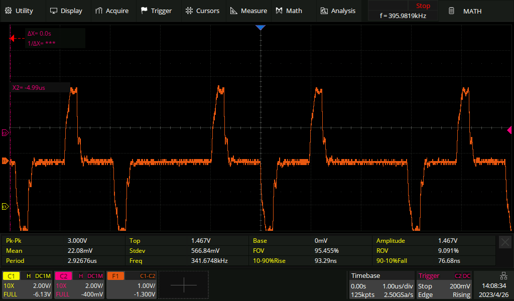
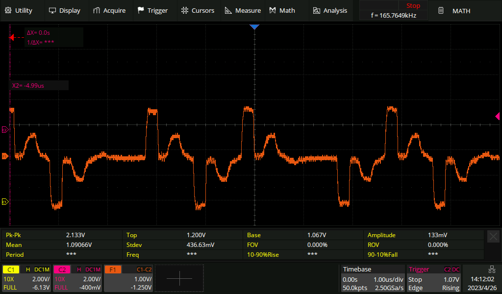
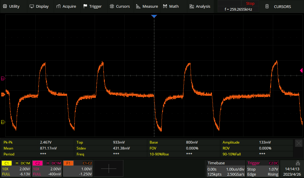
The post is based around Python code which transmits the packets, 'transmit_ss7.py', in the sample code which includes code in Python and C. The Python code transmits SS7 in all three of the major ways SS7 can be transmitted over an E1/T1 line: SS7 over ATM at 1536 kbit/s, SS7 over MTP-2 at 1536 kbit/s and then ordinary SS7 over 64 kbit/s MTP-2. Each one is transmitted for a few seconds.
SS7 over ATM
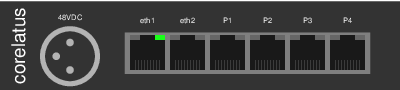
We're using an E1/T1 Messenger 3.0 with a loopback cable between P4 and P5:
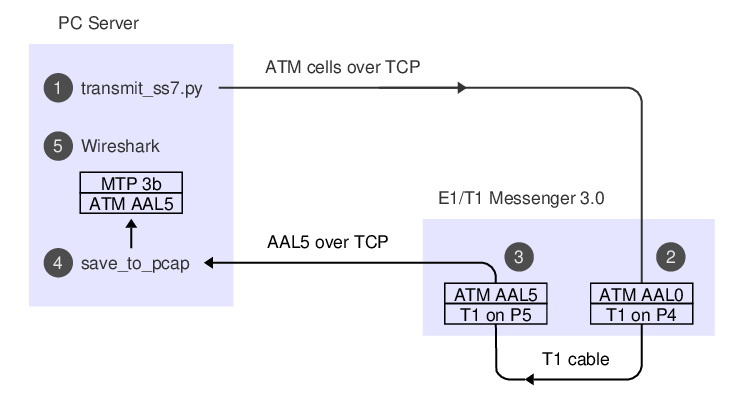
SS7 over ATM is specified in ITU-T Q.2110, Q.2111 and Q.2210. SS7 messages are sent from a lightly modified version of MTP-3 ("MTP-3b") over ATM AAL5. The Python code takes a couple of shortcuts: Instead of implementing AAL5, it uses hardcoded cells taken from unpublished test code. Instead of implementing the state machine from Q.2110 for link start-up, it just jumps in and starts transmitting.
To see the code running, set up some monitoring so we can observe the signalling we generate after it's taken a trip through the T1 cable. 'save_to_pcap' is in the same sample code repository as the Python code:
    ./save_to_pcap -l -p aal5 -a 0:5 172.16.1.10 4A 1-24 aal5_capture.pcapng
    monitoring 4A:1,2,3,4,5,6,7,8,9,10,11,12,13,14,15,16,17,18,19,20,21,22,23,24 interface_id=0
    capturing packets, press ^C to abort
Leave that code running in a window, it's going to capture packets which we send later.
The -l switch means 'assume layer 1 is already set up'.
-p aal5 and -a 0:5 means we want to decode AAL5 on VPI:VCI 0:5.
172.16.1.10 is the IP of the Corelatus hardware.
4A identifies the T1 interface, and 1-24 the timeslots.
To enable the T1 interfaces and run the Python code to transmit the SS7 signalling:
    ./gth.py 172.16.1.10 enable pcm4A mode T1
    ./gth.py 172.16.1.10 enable pcm5A mode T1
    ./transmit_ss7.py 172.16.1.10 5A
The 'save_to_pcap' code we ran as the first step will show some status changes:
    Mon Jun 23 15:15:14 2025 event: l1 message: name=pcm4A state=LFA
    Mon Jun 23 15:15:14 2025 event: l1 message: name=pcm5A state=LFA
    Mon Jun 23 15:15:14 2025 event: l1 message: name=pcm4A state=OK
    Mon Jun 23 15:15:14 2025 event: l1 message: name=pcm5A state=OK
    Mon Jun 23 15:22:10 2025 signalling job at5m4138 changed state to 'sync'
    Mon Jun 23 15:22:12 2025 signalling job at5m4138 changed state to 'hunt'
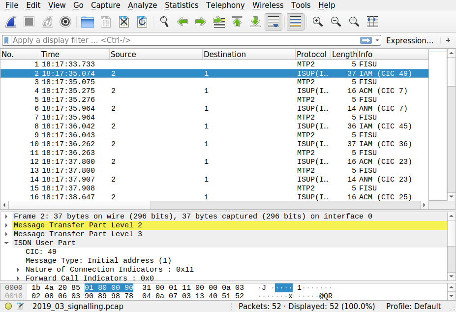
The signalling is now in 'aal5_capture.pcapng_00001'. Wireshark can display it in a GUI, tshark shows it as text:
    tshark -r ../c/aal5_capture.pcapng_00001
    1      0.000          DCE → DTE          SSCOP 33 Resynchronization
Regular SS7 over MTP-2
MTP-2 (ITU-T Q.703) has two main variants. The classic version sends the signalling on one 64 kbit/s timeslot. Then, Annex A provides an option to use all timeslots and thus send 1536 kbit/s on T1 or 1984 kbit/s on E1.
The API command 'fr_layer' does the actual transmission work: bit-stuffing, appending the frame-check-sequence (CRC) and delimiting the packet with flags. It also automatically repeats FISUs or LSSUs when there's nothing else to send.
To capture the signalling, use one of these two commands:
    ./save_to_pcap -l 172.16.1.10 4A 1-24 mtp2_high_speed.pcapng
    ./save_to_pcap -l 172.16.1.10 4A 1 mtp2_64kbit.pcapng
To transmit the signalling:
    ./gth.py 172.16.1.10 enable pcm4A mode T1
    ./gth.py 172.16.1.10 enable pcm5A mode T1
    ./transmit_ss7.py 172.16.1.10 pcm5A
The Python code sends two LSSUs, two MSUs and finally a FISU. Like the ATM code, it takes some shortcuts, e.g. it doesn't implement the state machines for starting up the link ("alignment") and retransmitting packets ("signal units").
'save_to_pcap' shows the status changes which happen when layer 1 is enabled and the Python code sends layer 2 packets:
    Mon Jun 23 15:33:26 2025 signalling job m2mo4139 changed state to 'out of service'
    Mon Jun 23 15:33:26 2025 signalling job m2mo4139 changed state to 'in service'
    Mon Jun 23 15:33:30 2025 signalling job m2mo4139 changed state to 'no signal units'
The resulting PCAP (Wireshark) file shows the five packets we sent:
tshark -r mtp2_high_speed.pcapng_00001
    1      0.000              →              MTP2 6 SIO
    2      1.000              →              MTP2 6 SIN
    3      2.003         5577 → 12099        MTP3MG (Int. ITU) 25 Unknown
    4      2.008            1 → 2            ISUP(ITU) 39 IAM (CIC 14)
    5      2.008              →              MTP2 5 FISU
Permalink | Tags: GTH, telecom-signalling
Decoding the telephony signals in Pink Floyd's 'The Wall'
Posted December 4th 2024
I like puzzles. Recently, someone asked me to identify the telephone network signalling in The Wall, a 1982 film featuring Pink Floyd. The signalling is audible when the main character, Pink, calls London from a payphone in Los Angeles, in this scene (Youtube).
Here's a five second audio clip from when Pink calls:
What's in the clip?
The clip starts with some speech overlapping a dial-tone which in turn overlaps some rapid tone combinations, a ring tone and some pops, clicks and music. It ends with an answer tone.
The most characteristic part is the telephone number encoded in the rapid tone combinations. Around 1980, when the film was made, different parts of the world used similar, but incompatible, tone-based signalling schemes. They were all based on the same idea: there are six or eight possible tones, and each digit is represented by a combination of two tones.
Let's examine a spectrogram
SoX, an audio editing tool for PCs, can make charts that show the spectral components of the audio over time. The horizontal axis represents time, the vertical axis frequency, and darker sections show more audio power, and lighter sections less.
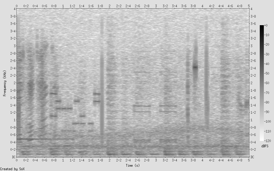
Signalling tones appear as dark horizontal lines in the spectrogram, with the digit signalling visible from 0.7 to 1.8 seconds. That part of the signalling has tones at roughly 700, 900, 1100, 1300, 1500 and 1700 Hz.
Which signalling standards were in common use?
DTMF (ITU-T Q.23 and Q.24)
Everyone's heard DTMF (Dual Tone Multi Frequency). It's the sound your phone makes when you interact with one of those "Press 1 if you are a new customer. Press 2 if you have a billing enquiry. Press 3..." systems. DTMF is still used by many fixed-line telephones to set up a call.
In DTMF, each digit is encoded by playing a "high" tone and a "low" tone. The low ones can be 697, 770, 852 or 941 Hz. The high ones 1209, 1336, 1477 and 1633 Hz.
None of the pairs in the audio match this, so it's not DTMF. Here's an audio clip of what it would sound like if we used DTMF signalling for the same number, with about the same speed of tones:
CAS R2 (ITU-T Q.400—490)
CAS R2 uses a two-out-of-six tone scheme with the frequencies 1380, 1500, 1620, 1740, 1860 and 1980 Hz for one call direction and 1140, 1020, 900, 780, 660 and 540 Hz for the other. None of these are a good match for the tones we heard. Besides, Pink is in the USA, and the USA did not use CAS R2, so it's not CAS.
This is what the digit signalling would have sounded like if CAS were used:
SS5 (ITU-T Q.153 and Q.154)
SS5 also uses a two-out-of-six scheme with the frequencies 700, 900, 1100, 1300, 1500 and 1700 Hz. This matches most of what we can hear, and SS5 is the signalling system most likely used for a call from the USA to the UK in the early 1980s.
This is what the digit signalling sounds like in SS5, when re-generated to get rid of all the other sounds:
SS7 (ITU-T Q.703—)
It can't be SS7. Signalling system No. 7 (SS7) doesn't use tones at all; it's all digital. SS7 is carried separately from the audio channel, so it can't be heard by callers. SS7 wasn't in common use until later in the 1980s.
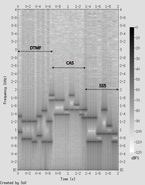
Comparing spectrograms
I made a spectrogram which combines all three signalling types on the same chart. The difference between DTMF and SS5 is subtle, but recognisable. CAS is obviously different.
Let's feed the audio to some telecom hardware
I injected the audio file into a timeslot of an E1 line, connected it to Corelatus' hardware and started an ss5_registersig_monitor.
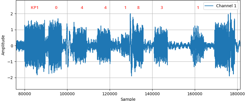
The input audio has a lot of noise in addition to the signalling, but these protocols are robust enough for the digital filters in the hardware to be able to decode and timestamp the dialled digits anyway. Now, we know that the number signalling we hear was 044 1831. The next step is to analyse the frequencies present at the start time for each tone. I re-analysed the audio file with SoX, which did an FFT on snippets of the audio to find the actual tone frequencies at the times there were tones, like this:
sox input.wav -n trim 0.700 0.060 stat -freq
The results are:
| Time | Frequencies | Interpretation |
|---|---|---|
| 0—1200 ms | 483 Hz | dial tone |
| 729 | 1105 + 1710 | KP1 (start) |
| 891 | 1304 + 1507 | 0 |
| 999 | 1306 + 703 | 4 |
| 1107 | 1306 + 701 | 4 |
| 1215 | 703 + 888 | 1 |
| 1269 | 902 + 1503 | 8 |
| 1377 | 902 + 1101 | 3 |
| 1566 | 701 + 900 | 1 |
| 1674 | 1501 + 1705 | ST (stop) |
| 3800 | 2418 | Answer tone |
At this point, I'm certain the signalling is SS5. It uses the correct frequencies to transmit digits. It uses the correct digit timing. It obeys the SS5 rules for having KP1 before the digits and ST after the digits. It uses a tone close to 2400 Hz to indicate that the call was answered.
I've also listed the dial tone at the beginning, and the 2400 Hz seizing tone at the end. SS5 also uses a 2600 Hz tone, which is infamous for its use in blue box phreaking (telephone fraud) in the 1980s.
How was the film's audio made?
My best guess is that, at the time the film was made, callers could hear the inter-exchange signalling during operator-assisted calls in the US. That would have allowed the sound engineer to record a real telephone in the US and accurately capture the feeling of a long-distance call. The number itself was probably made-up: it's too short and the area code doesn't seem valid.
The audio was then cut and mixed to make the dial tone overlap the signalling. It sounds better that way and fits the scene's timing.
Addendum, 18. December 2024: the audio also appears in 'Young Lust'
It turns out that an extended version of the same phone call appears near the end of 'Young Lust', a track on the album 'The Wall'. Other engineers with actual experience of 1970s telephone networks have also analysed the signalling in an interesting article with a host of details and background I didn't know about, including the likely names of the people in the call.
It's nice to know that I got the digit decoding right, we both concluded it was 044 1831. One surprise is that the number called is probably a shortened real number in London, rather than a completely fabricated one as I suspected earlier. Most likely, several digits between the '1' and the '8' are cut out. Keith Monahan's analysis noted a very ugly splice point there, whereas I only briefly wondered why the digit start times are fairly regular for all digits except that the '8' starts early and the final '1' starts late.
Addendum, 2. January 2025: what does a 'very ugly splice point' look like?
I wondered a bit about the "very ugly splice" Keith Monahan noted, so I took a look at the waveform of a FLAC copy of the 2011 remaster of Young Lust. Zooming in at the 193 second mark, the lack of an inter-digit pause between 1 and 8 is obvious, as is the unexpectedly large gap between the 3 and 1:
Here's what the waveform looks like when I zoom in on the area from the end of digit '1' to the start of digit '8':
I was expecting worse, but, back in 1979, audio splices were probably made by literally cutting magnetic tape with a razor blade, at a 45° angle, and scotch taping them back together, so perhaps that set an upper limit of ugliness which we can now easily surpass with digital splicing. Or maybe the splice was worse in the recording Keith had.
Permalink | Tags: GTH, telecom-signalling
How far can I place a PMP from the tap-in point? (update)
Posted May 9th 2023
In an earlier blog post, we took a look at what happens when we monitor an E1/T1 line with an incorrectly placed monitor point. In this post, we repeat the measurements with a high-quality oscilloscope.
What are we doing?
When monitoring an E1/T1 line in the standard (ITU-T G.772) way, you have a tap-in point and resistors near the tap-in point:
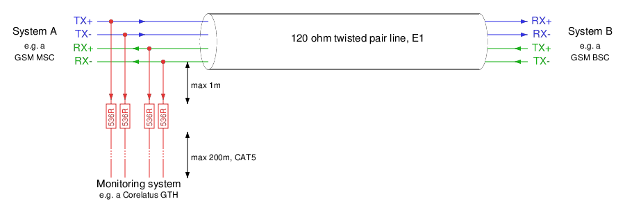
There are two distances marked on the schematic:
From the tap-in point to the resistors: this distance is critical. The shorter, the better.
From the resistors to the monitoring equipment: we have a lot of leeway. Tens of metres is normal, up to 200 metres is possible.
A practical lab monitor point
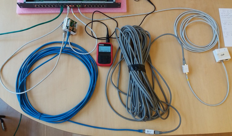
We created this demonstration in our lab with a live E1 link, and varied the cable lengths to demonstrate various effects on the signal.
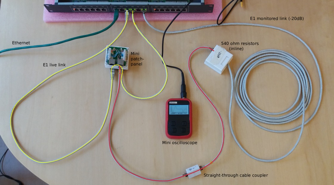
In the photo, we've got a pocket oscilloscope. For this post, we replaced the pocket oscilloscope with a 5 giga-sample/s Teledyne digital storage oscilloscope, to get better measurements. (That's way more than we need for an E1 line.)
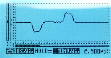
Live signal with a 0.5 metre tap-resistor distance
Here's what the live signal looks like in a correctly monitored setup, i.e. the one in the photo above.
The addition of the monitor point hasn't noticeably affected the live signal.
Live signal with a five metre tap-resistor distance
If we extend the tap-in to resistor distance to five metres, then the live signal becomes noticeably affected. The pulse has become slightly deformed, especially on the trailing edge. If the live link was extremely long haul, then we might be unlucky enough to cause it to go from "barely works" to "no longer reliable".
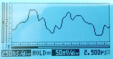
Live signal with a 50 metre tap-resistor distance
If we keep going and extend the distance to 50 metres, the live signal is now affected to the point that it'll no longer work reliably. We can see an extra pulse after every real pulse:
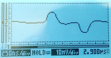
Live signal on a long haul line
All of the above measurements were made with a short live E1 line, only a metre or two. For comparison, here's what an E1 looks like after 200 metres of cable. The pulses become shark-fin like. The receiving equipment expects this and has no trouble decoding the signal.
Permalink | Tags: GTH, telecom-signalling
Reading SS7 packets from a PCap file and replaying
Posted March 25th 2019
This is the second in a three-part series about different ways to replay signalling on an E1/T1 line in the lab. The three parts are:
- Replaying a bit-exact recording of an E1 timeslot.
- Reading SS7 packets from a .pcap file, re-create layer 2. (this post)
- Creating SS7 packets from scratch.
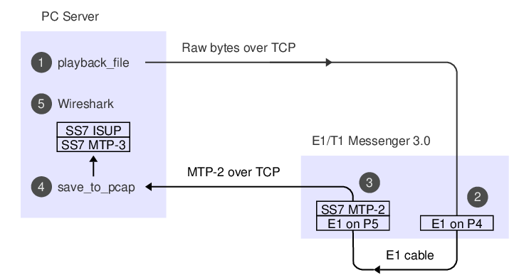
This post is about the second approach. It's particularly useful because we can use this technique to convert a SIGTRAN capture into an SS7 capture with MTP-3 and MTP-2. It's also satisfying because we can take packets full circle—we can play the packets from a PCap file and make a new PCap file with the same packets after they've passed through an E1 line. It assumes you have an E1 cable between P5 and P6, as illustrated in the previous post on this subject.
Approach #2: Read packets from a PCap file, replay on E1
Here's what the data-flow looks like:
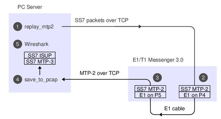
1. The 'replay_mtp2' program reads SS7 packets from a PCap file.
2. The Corelatus box does bit-stuffing and inserts flags and FISUs.
3. After the signal goes out through an E1 cable and back in again,
the Corelatus box recovers the SS7 packets.
4. 'save_to_pcap' saves the packets in PCapNG format.
5. Wireshark decodes MTP-3 and higher SS7 layers to display the packets.
The API command 'fr_layer' does step 2, it's described in the API manual. Here's what we do if we're using the C sample code:
    ./enable 172.16.1.10 pcm5A
    ./enable 172.16.1.10 pcm6A
    ./replay_mtp2 gth30 isup_load_gen.pcapng 5A 16
The PCap file with the signalling was made by a load generator. We can capture the signalling and make a new PCap file with the same packets, like this, in a separate window:
    ./save_to_pcap  -l 172.16.1.10 6A 16 gth.pcapng
    monitoring 6A:16 interface_id=0
    capturing packets, press ^C to abort
    saving to file gth.pcapng_00001
    Fri Mar 15 17:17:34 2019 signalling job m2mo0 changed state to 'in service'
    Fri Mar 15 17:17:48 2019 signalling job m2mo0 changed state to 'no signal units'
    ^C
We can view both files in Wireshark and compare them. They'll contain the same packets, but with different relative timing, since 'replay_mtp2' just replays the packets as fast as possible.
Replaying other files
Wireshark has a collection of SS7 capture files, with all sorts of contents. They're all in the old 'classic' PCap format, so we have to convert them.
isup.cap
This file has three challenges. First, it's in the old PCap format. Second, the transport is SIGTRAN, so we have to extract the MTP-3 packets. Third, it uses a pre-RFC version of M3UA, so it's hard to see where the MTP-3 packets are. By inspecting the hex dump, we can see that MTP-3 starts 74 bytes into each packet, so we can use 'editcap' to make a new PCap file and then play it:
    > editcap -L -C 74 -T mtp3 isup.cap isup_fixed.pcap
    > ./replay_ss7 172.16.1.10 isup_fixed.pcap 5A 16
   Found link type 141 in capture file
   packet bytes replayed: 158. Sleeping to drain buffers.
Here's what the contents look like after a round-trip through the E1:
    >tshark -r mml.pcap_00001
    1      0.000        11522 ->        ISUP(ITU) 77 IAM (CIC 213)
    2      0.003        12163 -> 11522        ISUP(ITU) 21 CFN (CIC 213)
    3      0.005        12163 -> 11522        ISUP(ITU) 17 ACM (CIC 213)
    4      0.007        12163 -> 11522        ISUP(ITU) 17 ANM (CIC 213)
    5      0.010        11522 -> 12163        ISUP(ITU) 21 REL (CIC 213)
    6      0.012        12163 -> 11522        ISUP(ITU) 17 RLC (CIC 213)
    7      0.013              ->              MTP2 5 FISU
If you look at the output file more closely, you can see that the MTP-2 fields are faked; the sequence numbers don't increment. That's because the original data didn't have any sequence numbers in it. If we wanted to, we could extend 'replay_ss7' to generate realistic sequence numbers.
camel.pcap and camel2.pcap
These are more classic PCap files with SIGTRAN, but again we can convert them:
    > editcap -L -C 74 -T mtp3 camel.pcap camel_fixed.pcap
    > ./replay_ss7 172.16.1.10 camel_fixed.pcap 5A 16
   Found link type 141 in capture file
   packet bytes replayed: 559. Sleeping to drain buffers.
Viewing it in Wireshark requires "Signalling Connection Control Part"/"Protocol Preferences"/"Default Payload" to be set to TCAP. Same thing in 'tshark':
    >tshark -o "sccp.default_payload: tcap" -r mml.pcap_00001
    1      0.000           10 -> 100          Camel-v2 165 invoke initialDP
    2      0.027          100 -> 10           Camel-v2 217 invoke requestReportBCSMEvent invoke applyCharging invoke continue
    3      0.034           10 -> 100          TCAP 57 Continue otid(06f7) dtid(13b8)
    4      0.045           10 -> 100          TCAP 85 Continue otid(ec0f) dtid(0d7c)
    5      0.051          100 -> 10           TCAP 45 End dtid(ec0f)
    6      0.052              ->              MTP2 5 FISU
gsm_map_with_ussd_string.pcap
Same encoding as the 'camel' files. Contents:
    >tshark -r mml*
    1      0.000         1041 -> 8744         GSM MAP 149 invoke processUnstructuredSS-Request
ansi_map_ota.pcap
    editcap -L -C 82 -T mtp3 ansi_map_ota.pcap ansi_fixed.pcap
    ...
    >tshark -r mml*   // after a round-trip through E1:
    1    0.000  18 -> 10  ANSI MAP 81 SMS Delivery Point to Point Invoke
    2    0.009  10 -> 18  ANSI MAP 69 SMS Delivery Point to Point ReturnResult
    3    0.020  18 -> 10  ANSI MAP 85 SMS Delivery Point to Point Invoke
    4    0.026  10 -> 18  ANSI MAP 45 SMS Delivery Point to Point ReturnResult
    5    0.036  18 -> 10  IS-683 81 SMS Delivery Point to Point Invoke
japan_tcap_over_m2pa.pcap
This file uses the Japanese variant of MTP-3. We need to tell Wireshark about that in the MTP-3 preferences:
    editcap -L -C 79 -T mtp3 japan_tcap_over_m2pa.pcap japan_fixed.pcap 2 4 6
    ...
    >  tshark -o "mtp3.heuristic_standard: TRUE" -r /tmp/mml.pcap*
    1      0.000         3003 -> 2730         SCCP (Japan) 32 SSA
    2      0.009         2730 -> 3003         TCAP 72 Begin otid(18250001)
    3      0.016         3003 -> 2730         GSM MAP 56 returnResultLast Unknown GSM-MAP opcode
ansi_tcap_over_itu_sccp_over_mtp3_over_mtp2.pcap
This is the only SS7 capture on the Wireshark Sample Captures page which actually captured MTP-2. The hardware that captured it didn't save the FCS (Frame Check Sequence, a 16-bit CRC), so we need to tell 'replay_ss7' about that, otherwise the last two bytes of each packet will be chopped off:
    tshark -r ansi_tcap_over_itu_sccp_over_mtp3_over_mtp2.pcap ansi_fixed.pcap
    ./replay_ss7 -f 172.16.2.8 ansi_fixed.pcap  5A 16
    ...
    >  tshark -r /tmp/mml.pcap*
    1      0.000         9283 -> 9444         ANSI MAP 150 Origination Request Invoke
Skipped files
I didn't bother with a few of the sample captures in the Wireshark wiki.
'bicc.cap' only contains one packet and it's not SS7.
'ansi_map_win.pcap' contains truncated packets.
'packlog-example.cap' contains a hex dump of a few packets,
in a pinch we could convert it with 'text2pcap'.
Permalink | Tags: GTH, telecom-signalling
Replaying bit-exact E1/T1 timeslot recordings
Posted March 15th 2019
This note is about replaying signalling on an E1/T1 line in the lab, using an E1/T1 Messenger 3.0. We can connect two ports with a yellow crossover cable to make the Corelatus system talk to itself over an E1/T1 link.

Now that we've connected two E1 (or T1) ports, we can transmit and receive bytes. The next step is to make suitable bytes for transmission. Depending on what we have and what we want to do, we can use choose between three techniques:
- Replaying a bit-exact recording of an E1 timeslot. (this post)
- Reading SS7 packets from a .pcap file, re-create layer 2.
- Creating SS7 packets from scratch.
This post is about the first approach. I'll cover the other two in later articles.
Approach #1: bit-exact record-and-replay
We can record an E1 timeslot at an operator, take the file back to the lab and then replay it while working on the code to decode the SS7 packets we're interested in. Using a bit-exact recording lets you reproduce what happened in the operator's network. The relative packet timing will be the same. The sequence numbers will be identical. The packet payload will be identical.
All Corelatus hardware can record bit-exact timeslots, both on electrical E1 lines and on optical fiber (E1-on-SDH).
To replay, you need an E1/T1 Messenger 3.0, because it has transmit capabilities. If you have a E1/T1 Monitor 3.0, i.e. listen-only, you can temporarily turn it into a Messenger with a firmware update.
Here's what the data-flow looks like:
The API commands needed for the recording and replaying, respectively, are 'recorder' and 'player'. They're described in the API manual, e.g. under 'new player'. We'll just use the C version of the sample code. If you prefer, you can use the Python or Perl version, or hack up your own code.
Here's how you can record a timeslot:
    ./record -l 172.16.1.10 1A 16 /tmp/signalling.raw
    started recording. Press ^C to end.
    0 1448 2896 4096 5544 6992 8192 9640 11088 ^C
The -l switch tells record that L1 is already set up, that way we avoid resetting it.
Back in the lab, we can replay the signalling file we made earlier. I've linked to a copy so you can try it. First, we need to turn the E1 ports on:
    ./enable 172.16.1.10 pcm5A
    ./enable 172.16.1.10 pcm6A
The LEDs in the ports will turn to green and the built-in webserver shows the ports as being in status OK. Next step is to replay the bits, i.e. step (1) on the data flow diagram:
    ./playback_file -l 172.16.1.10 5A 16 /tmp/2019_03_signalling.raw
    0 1600 3200 4800 6400 8000 wrote 8192 octets to the player
    all done
Most likely, you want to decode the signalling while playing it, this is step (4) on the diagram. You can do that in a separate window, like this:
    ./save_to_pcap  -l 172.16.1.10 6A 16 gth.pcapng
    monitoring 6A:16 interface_id=0
    capturing packets, press ^C to abort
    saving to file gth.pcapng_00001
    Fri Mar 15 17:17:34 2019 signalling job m2mo0 changed state to 'in service'
    Fri Mar 15 17:17:48 2019 signalling job m2mo0 changed state to 'no signal units'
    ^C
When you've captured enough, hit control-C and view the PCap file with Wireshark, which is step (5) on the dataflow diagram. It'll look something like this:
Permalink | Tags: GTH, telecom-signalling
Figuring out a Corelatus module's (forgotten) IP address
Posted July 3rd 2017
If you have a Corelatus module but don't know what the IP address is, you can figure it out by power cycling and then sniffing on UDP port 9—a newly booted module will broadcast its address every couple of minutes. The broadcasts stop as soon as you connect to the module's HTTP server (port 8888), the API (port 2089) or the SSH CLI.
Step by step
To do this, you need a laptop with an ethernet port, an ethernet cable and software to sniff ethernet. In this post, I'm using a 'Thinkpad 13' with a USB ethernet dongle, running Linux. I sniff the packets with 'tcpdump'. 'Wireshark' works well too, especially with Windows.
1. Connect the ethernet cable
Plug the the ethernet cable in to 'eth1' on the Corelatus module and in to the ethernet port on your laptop. In less than a second, the ethernet link is established and the LEDs for 'eth1' on the Corelatus module will look like this:
By connecting the ethernet cable directly instead of through a switch, router or gateway, we can be sure that we're seeing exactly what comes out of the Corelauts module and we can also be sure that nothing else will try and control the module.
2. Figure out which ethernet port to sniff on
Many laptops have multiple ethernet interfaces. Here's one way to list them:
  matthias@eldo:~$ sudo ifconfig
  enp0s31f6: flags=4099 UP,BROADCAST,MULTICAST  mtu 1500
  ether 54:ab:3a:a5:47:e7  txqueuelen 1000  (Ethernet)
  RX packets 0  bytes 0 (0.0 B)
  RX errors 0  dropped 0  overruns 0  frame 0
  TX packets 0  bytes 0 (0.0 B)
  TX errors 0  dropped 0 overruns 0  carrier 0  collisions 0
  device interrupt 16  memory 0xf1100000-f1120000

  enx98ded01f64bc: flags=4099 UP,BROADCAST,MULTICAST  mtu 1500
  ether 98:de:d0:1f:64:bc  txqueuelen 1000  (Ethernet)
  ...
Another way to list them is with 'tcpdump --list-interfaces'. In 'wireshark', there's a menu which shows the same thing. If there are multiple Ethernet interfaces, you can either take an educated guess as to which is the wired port, or just try each one in sequence.
3. Start sniffing
With 'tcpdump', these commands work well:
  matthias@eldo:~$ sudo ifconfig enx98ded01f64bc up

  matthias@eldo:~$ sudo tcpdump --interface=enx98ded01f64bc -n -X port 9
  tcpdump: verbose output suppressed, use -v or -vv for full protocol decode
  listening on enx98ded01f64bc, link-type EN10MB (Ethernet), capture size 262144 bytes
I've restricted the capture to the wired interface, 'enx98...', to avoid being distracted by a flood of packets from WiFi.
4. Cycle power on the Corelatus module
Remove all power to the Corelatus module. Then plug power back in. A cold boot takes about 40 seconds. After a further 60 seconds, the module will send a broadcast packet which shows its IP address:
  23:24:18.492770 IP 172.16.2.5.57255 > 172.16.255.255.9: UDP, length 65
  0x0000:  4500 005d 0000 4000 4011 e06a ac10 0205  E..]..@.@..j....
  0x0010:  ac10 ffff dfa7 0009 0049 bc09 4754 4820  .........I..GTH.
  0x0020:  7069 6e67 2e20 5365 6520 6874 7470 3a2f  ping..See.http:/
  0x0030:  2f77 7777 2e63 6f72 656c 6174 7573 2e63  /www.corelatus.c
  0x0040:  6f6d 2f67 7468 2f66 6171 200a 4d61 736b  om/gth/faq..Mask
  0x0050:  3a20 3235 352e 3235 352e 302e 30         :.255.255.0.0
The packet above shows that the IP address is 172.16.2.5. The last line of the capture also tells us that the network mask is 255.255.0.0.
Finding the bad link in an SDH network using BIP counters
Posted June 15th 2017
SDH/SONET has relatively powerful mechanisms for detecting transmission errors, far better than E1/T1 lines. We can use those mechanisms to figure out which optical link in a network has errors. This post shows which parts of the network can see errors in various cases—and which parts cannot.
SDH error detection and counters
SDH packs data into virtual containers (VCs). VCs can be nested, for instance an E1 is transported using a VC-12 and up to 63 VC-12s can in turn be packed together into a larger container called a VC-4. Each of those containers has parity bits so that the receiver can see if the data was damaged in transit. These parity bits are called a bit interleaved parity (BIP).
Each add/drop multiplexor (ADM) in an SDH network keeps count of the number of errors in each BIP it checks. Normally, the ADM will only check the BIP in a container it unpacks or re-packs. Each ADM also sends reports of the BIP error counts backwards on each link. Such a report is called a remote error indication (REI).
By looking at BIP counters and REI counters in various parts of the network, we can reason about the likely source of transmission errors.
A concrete example: case 1
On the left side of this network, we have 15 E1s. They are transported along the light blue path over to the right side of the diagram:
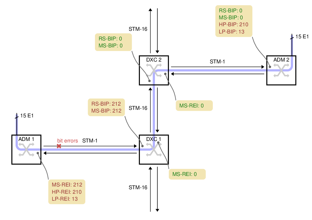
ADM 1
ADM 1 picks up 15 electrical E1s and packs them into 15 VC-12 containers. The VC-12s are packed into a VC-4 and transmitted over a 155 Mbit/s STM-1 optical link towards the operator's core network.
For this case, we're assuming the fiber between ADM 1 and DXC 1 has a problem which causes bit errors. The problem spot is marked with a red cross on the fiber. DXC 1 is in the best position to detect those bit errors since it is directly connected to the fiber with the problem.
DXC 1
DXC 1 is a high-capacity digital cross-connect which can forward data to the operator's 2.5 Gbit/s STM-16 ring. Some manufacturers abbreviate digital cross-connect system to DXC, others use DCS.
The DXC counts two types of parity errors on the incoming fiber: RS-BIP and MS-BIP (Regenerator Section and Multiplex Section Bit Interleaved Parity). Both count an estimate of the number of bit errors in (almost) the whole STM-1. In this example, 212 errors have been detected by both counters, the diagram shows them in yellow boxes.
DXC 1 also transmits the error counts back to ADM 1, as remote error indication (REI) values. They are shown in the yellow box below each node.
DXC 2
DXC 2 cannot report any transmission errors. The DXC's switching granularity is a whole VC-4, so it never unpacks the VC-4 or VC-12s to check the BIPs. DXC 2 just forwards an exact copy of the incoming VC-4.
ADM 2
ADM 2 unpacks both the VC-4 and all 15 VC-12s, so it can report the HP-BIP (High-order Path, Bit Interleaved Parity) and the LP-BIP (Low-order Path) errors. In this example, 210 errors were detected in the HP-BIP and 13 in the LP-BIP.
A more complicated example: case 2
In this example, two ADMs are connected in series on the left, with each one attaching several E1s to the SDH network:
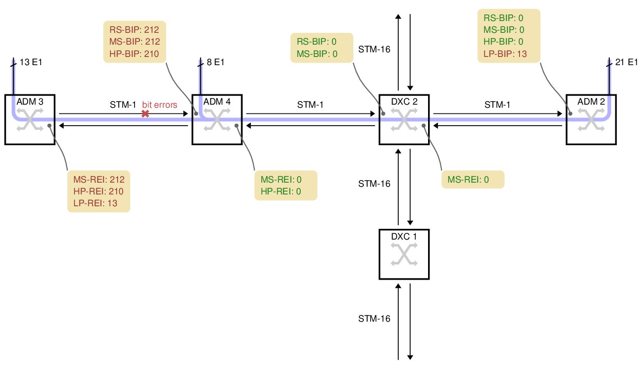
ADM 3 has 13 E1s which it sends rightwards. For this example, the bit errors are on the fiber between ADM 3 and ADM 4, marked with a red cross.
ADM 4 has a further 8 electrical E1s. It unpacks the 13 VC-12s from ADM 3, adds the 8 new VC-12s, makes a new VC-4 and transmits the result to DXC 2.
DXC 2 cannot report any errors because it just copies the incoming VC-4.
ADM 2 unpacks all 21 E1s, so it can see that 13 of the LP-BIP counters have errors, but 8 do not. Armed with a map of the network, this is often enough information to deduce where the problem is. There are no HP-BIP errors, however, because the VC-4 arriving here was made by ADM 4, whereas the transmission errors happened before ADM 4.
Practical Complications
All ADMs and DXCs are capable of counting the number of BIP errors down to the level above their switching granularity. But actually finding the value in the manufacturer's command-line or GUI is not always easy. On Corelatus equipment, the values are displayed on the on-board HTTP server, under SDH. They are also available via the CLI and API.
The names for the BIP error counters vary from manufacturer to manufacturer. Sometimes, the counter is named after the byte in the SDH frame the counters are carried on, i.e. B1, B2, B3 and V5 correspond to RS-BIP, MS-BIP, HP-BIP and LP-BIP, respectively.
When Corelatus equipment is used with SONET, it reports the counters using the standard SONET names, e.g. REI-L for what would be called MS-REI in SDH.
Using an optical splitter, you can always connect a Corelatus SDH Monitor 3.0 to an STM-1 link and see the BIP and REI counters at all levels. That provides more information about errors than just looking at a DXC's counters, partly because the Corelatus system can report BIP errors all the way down to VC-12 and partly because the Corelatus system can decode and record the data on E1/T1 timeslots. In case 2, the DXC does not report the LP-BIP errors because the DXC has no reason to unpack the VC-12s it is carrying, but a Corelatus system connected any of fiber links along the whole transmission path will report the LP-BIP errors and, optionally, decode SS7 or other signalling on individual E1 timeslots.
Permalink | Tags: GTH, telecom-signalling, SDH and SONET
What does an improperly placed monitor point do to a signal?
Posted August 19th 2016
There is a standardised way to monitor E1/T1 links. It is defined in ITU-T G.772 and is formally called a "Protected Monitoring Point". A correctly installed protected monitor point doesn't disturb the live link. This blog entry is about what happens if you install a monitor point incorrectly.
Update: we repeated the measurements in this post, using a high-quality oscilloscope.
A protected monitor point (in theory)
A G.772 protected monitoring point connects to a live line in such a way that the live line is protected from three common fault conditions after the monitoring point:
- An unterminated line, for instance by inadvertently leaving a cable unplugged.
- A short circuit.
- Unintentional transmission, for instance if the monitoring line is accidentally connected to another transmission line, or if monitoring equipment is accidentally mis-configured to transmit.
Here's one way to build a protected monitor point on an E1 line:
There's an important note on the schematic: "max 1m" cable from the tap-in point to the resistors in the monitor point. The shorter the distance from the tap-in point to the resistors, the better. In many cases, it's possible to mount the resistors just a few millimetres from the tap-in point.
A practical lab monitor point
To demonstrate what happens to an E1 signal, we created a live link in our lab, with connections just like in an operator's network. We've used a 1m long cable, the maximum allowed, from the tap-in point to the resistors. We then looked at the signal using a low-cost handheld oscilloscope.
The chassis at the top of the photo is a Corelatus Messenger 2.1 with three modules in it. Messenger is normally used as an active part of an E1 network, e.g. to implement a voicemail system. We're only using the center module, which has two ethernet ports and eight E1/T1 ports. The green cable is the ethernet cable used to control the system.
The yellow line is the live E1 link. It goes from port 'pcm1A' to a break-out box with punch blocks and then on to port 'pcm2A'. We can measure the number of bit errors on the live link. The punch blocks are the same as the ones operators have mounted in racks in their distribution frames.
The red line taps in to the live E1 link at the punch blocks. The length of this red line is critical: if it's too long then signal reflections from the 536 ohm resistors at the end of the red line will disturb the live link. Corelatus specifies a maximum length of 1m for this red line, in the above example we've used two 0.5m cables. In examples further down the page, we'll increase that to see how bad things can get. The red line leads to a box containing the monitoring resistors and then a 5m long cable back to the Messenger 2.1, where we've configured the incoming port to expect an attenuated signal. The length of the cable from the resistors to the monitoring equipment is not critical, it can be up to 200m.
Here's what the signals on this setup look like. On the left, the live signal and on the right the monitored signal, which is attenuated by 20dB. Both signals are clean and have the expected shape.
The scope indicates the scale on-screen; the horizontal (time) scale on both is the same, the vertical scales are different. We're measuring through an x10 oscilloscope probe in all cases.
Extending the red line to 10m
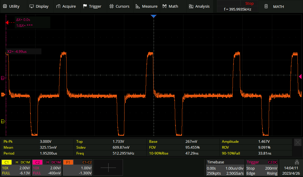
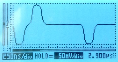
A 10m long tap line is out of spec. A real installation should not have such a long tap line. We expect the signal to go from the tap-in point, partially bounce from the resistor box and then interfere with the live signal. The time for a signal to travel down a 10m line, bounce, and travel back up again is approximately 100ns. 100ns is roughly one third of a division on the scope image, so we expect the damage to be that pulses change shape, rather than new pulses appearing between real pulses. The scope images show that the live signal (left) is damaged, whereas the monitored signal (right) is hardly affected:
Extending the red line to 35m
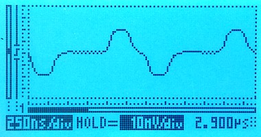
Using a 35m long cable to tap in will give a reflection after approximately 350ns. The damage to the live signal is severe, but the monitored signal still looks mostly OK:
The disturbance on the live link is so severe that the live link fails completely. Framing is lost; moving the live link from status "OK" to "LFA" and several other layer 1 error counters (e.g. code violation) increase rapidly. Another simple indication that the link has failed is that the LEDs on the live link have changed colour to orange, they're visible at the top of this photo:
Probing E1 lines with an oscilloscope
The proper way to measure balanced E1 signals in the lab is with a two-channel oscilloscope, with one probe on each of the E1's conductors. The scope can then display the result in differential, i.e. A-B, mode, with no risk of accidentally grounding one side of the E1.
Since the Vellemann oscilloscope only has one channel, there's no A-B mode. So we have no choice but to connect the probe's "ground" to one conductor and the probe's tip to the other. This works fine, and there are no concerns about grounding since the scope is normally battery powered.
The Velleman oscilloscope is cheap and this was the first time we used it, so we checked the measurements using a high quality analog oscilloscope, a Tektronix 2445. The measurements agree well.
We were pleasantly surprised by the Vellemann oscilloscope. It's by far the cheapest Distrelec have, but it works nicely. We left it in the default 'auto' mode and just pressed the 'hold' button a few times for each measurement to get a trace with a couple of pulses in it. It's easily small and cheap enough to take along to a site. (Corelatus has no association with Vellemann or Distrelec, except as a customer. We recommend this scope because it is useful in our experience. We're not paid to recommend it.)
Permalink | Tags: GTH, telecom-signalling
Debugging a PDH frequency offset
Posted March 6th 2016
Once or twice a year, I debug a network problem which turns out to be caused by a bad synchronisation topology. Here's how I debugged the most recent one.
Symptoms
The direct way to see a frequency offset in a PDH network is to measure the frequency at different interfaces in the network, preferably to an accuracy of at least fractional ppm. The frame rate on an E1 line is supposed to be exactly 8 kHz. But... normally, we see less direct symptoms.
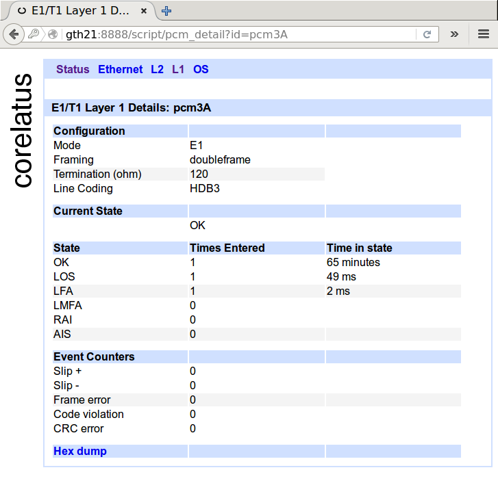
One indirect symptom is clearly visible in the layer 1 counters. Below is a screenshot of normal layer 1 counters for an E1. In cases where there's a frequency offset, you'll see the 'slip +' or 'slip -' counters increasing at a rate of about one per minute, or faster, depending on how bad the frequency offset is.
Another indirect symptom is visible in the layer 2 counters of some, but not all, protocols. E.g. in SS7 MTP-2, almost every slip causes a packet to be damaged, so you can see the errored signal unit(ESU) counter increase at a rate of a few per minute. ISDN LAPD, on the other hand tends to hide hide slips, especially at low load.
Analysing a recording
In this case, we could see the SS7 MTP-2 ESU counter increase at an abnormal rate on some timeslots, so I asked for a recording of a couple of minutes of one of the SS7 MTP-2 signalling timeslots which had damaged signalling. Corelatus hardware lets you make bit-exact recordings of live timeslots, either through the HTTP interface or using the 'record' program in the C sample code.
With the recording in hand, I started off by playing it back on a reference GTH 2.1 in our lab, effectively making a copy of the live link in our lab. Turning on MTP-2 decoding, here's what I saw:
| Packet | Time (milliseconds) | Packet dump |
|---|---|---|
| 1 | 0 | 84 9a 00 6c 4d |
| 2 | 134 | 85 9a 00 b0 17 |
| 3 | 2107 | 85 9a b0 17 |
| ... | ||
| 20 | 17921 | 86 a2 00 b6 80 |
| 21 | 22125 | 86 a2 00 86 |
| ... | ||
| 29 | 37351 | 86 a6 00 d6 e7 |
| 30 | 41540 | a6 00 d6 e7 |
SS7 MTP-2 links in normal operation carry nonstop packets: when there's nothing useful that needs to be sent, they send a five octet fill-in signal unit (FISU) over and over again. FISUs are always five octets long and they always have 00 as the middle octet.
Looking at the packet dump, packets 1, 2, 21 and 29 are all valid FISUs. Packets 3, 21 and 30 are all invalid---they are too short to be valid MTP-2 packets and they have incorrect CRCs (frame check sequence). It's pretty easy to see that each bad packet is just like its predecessor, except that one octet has been deleted.
(Aside: if you look closely, the defect in packet 21 isn't exactly a deleted octet. That's because MTP-2 uses bit stuffing and isn't octet aligned. We'll ignore that for now.)
A missing octet is a smoking gun for 'slips'
Having one missing octet in a packet is a smoking gun for a 'negative slip': different parts of the operator's PDH network are running at different frequencies, which forces layer 1 to compensate by throwing out a byte every so often. The missing octet rules out other possible causes for packet damage, in particular bit errors.
At this point, the evidence is already strong, but we can add one more thing to make it overwhelming: look at the elapsed time between damaged packets. We expect 'slip' events to be periodic. Between packets 3 and 21, the elapsed time is 20018ms. Between packets 21 and 30, the elapsed time is 19415ms.
From the elapsed time, we can estimate the frequency difference in the mis-synchronised parts of the network. An E1 timeslot is supposed to carry exactly 8000 octets per second, which corresponds to 125 microseconds per octet. A deleted octet every 20s or so corresponds to a frequency error of 6ppm.
In this case, we're seeing negative slips. The reverse is also possible. In a 'positive slip', layer 1 repeats an octet every so often.
Fixing the root cause
At the time of writing, I don't know what the root cause is. But I can offer a guess based on experience: part of the operator's PDH network has lost contact with the operator's primary reference clock, probably because of a configuration error in one or more cross-connects or MUXes in the network.
A primary reference clock is supposed to maintain long-term accuracy to 1 part per 1011 (ITU-T G.811). The frequency offset we can observe in the spacing of the slips is about 6 parts per 106 (6 ppm), i.e. many orders of magnitude worse than intended.
Permalink | Tags: GTH, telecom-signalling
Decoding random data
Posted March 13th 2015
If you were to feed a timeslot random data and try to decode that as though it were MTP-2, how long would it take until you get a valid packet?
(Quick answer: it'll happen about once every week or two on a regular 64kbit/s link.)
What does it take for a packet to be valid MTP-2?
If we send random data, then every so often there's going to be a flag. That signals start- and end-of-packet for MTP-2, so random data will look like it has packets. But to get valid packets, there are several more hoops to jump through:
- The CRC must be right.
- The packet must be a multiple of 8 bits long, e.g. 31 bit packets aren't allowed.
- The length indicator must be right.
- The packet must be between 5 and 272 octets (bytes) long.
It's possible to calculate how often all of those requirements are met...but it seems easier and less prone to "oh, I didn't think of that" to just try it and see what happens.
Test setup
I used a Corelatus E1/T1 Messenger 2.1 with a crossover E1 cable so that everything it transmits on one E1 port is received on another. I didn't write any code to do this, I just used programs from the C sample code collection, like this:
      $ ./playback_file 172.16.2.7 3A 1 /dev/urandom
      // in another window
      $ ./save_to_pcap 172.16.2.7 4A 1 /tmp/random.pcap
Results
After about 12 hours, the MTP-2 counters looked like this:
| Interface | Timeslot | Status | MSUs | ESUs | FISUs | LSSUs | Load % |
|---|---|---|---|---|---|---|---|
| 4A | 1 | no signal units | 3 | 10964728 | 0 | 0 | 0 |
We got 11 million bad packets and 3 good ones and no FISUs. Looking at the "good" ones more closely, it's obvious that they're not good either. Here's one of them:
      $ tshark -x -r /tmp/random.pcap | tail -2
      0000  9e e2 49 ef a1 95 0f b0 7a 34 b6                  ..I.....z4.

      $ tshark -V -r /tmp/random.pcap
      Frame 3: 11 bytes
      Interface id: 0 (4A:1)
      Encapsulation type: SS7 MTP2 (42)
      Arrival Time: Mar 13, 2015 11:36:56.057000000 CET
      Message Transfer Part Level 2
      .001 1110 = Backward sequence number: 30
      1... .... = Backward indicator bit: 1
      .110 0010 = Forward sequence number: 98
      1... .... = Forward indicator bit: 1
      ..00 1001 = Length Indicator: 9
      01.. .... = Spare: 1
      Message Transfer Part Level 3
      Service information octet
      11.. .... = Network indicator: Reserved for national use (0x03)
      ..10 .... = Spare: 0x02
      .... 1111 = Service indicator: Spare (0x0f)
      Routing label
      .... .... .... .... ..01 0101 1010 0001 = DPC: 5537
      .... 0000 0000 1111 10.. .... .... .... = OPC: 62
      1011 .... .... .... .... .... .... .... = Signalling Link Selector: 11
      Data: 7a34b6
Two things aren't quite right. First, the spare bits are normally set to zero (but Q.703 doesn't require this). Second, the length indicator is 9, but should be 6 for this packet (Q.703 requires checking this; Corelatus GTH accepts it anyway to make it easier to debug installations which use extended sequence number format).
Permalink | Tags: GTH, telecom-signalling, SDH and SONET
I have 47 E1s? How much hardware do I need to monitor them?
Posted January 14th 2015
Updated 6. February 2018 because of capacity improvements in hardware shipped from this date onwards: we have improved MTP-2 decoding capacity from 96 channels to 240 channels.
A common question when starting a monitoring project is "how much
hardware do I need to monitor these E1 (or T1) lines?". The final
word is always the specifications:
E1/T1 Monitor 3.0
SDH Monitor 3.0
One way to get started is to look at some real-world examples:
Example 1: 47 E1 lines, each with one 64 kbit/s SS7 MTP-2 signalling link
This is a classic E1 setup. Each E1 carries 30 timeslots of voice and one timeslot of signalling. In this example, we'll assume:
- The 30 subscriber timeslots (normally voice) on each E1 are not of interest. We can ignore them.
- We want both directions of the signalling.
To monitor that, we need enough ports to plug all the E1s into, and we need enough capacity to decode the MTP-2 signalling.
Ports: An E1/T1 Monitor 3.0 has 64 E1 receivers (spec. 2.1.1). The site in this example has 47 E1 lines, but we want both directions of them, so we need 2 x 47 = 94 E1 receivers. So we'll need two E1/T1 Monitor 3.0. We can plug the first 32 E1s into one and the remaining 15 into the other.
MTP-2 decoding capacity: An E1/T1 Monitor 3.0 can monitor 240 simplex ordinary 64 kbit/s MTP-2 channels (spec. 2.2.1). The site has 94 channels. So dimensioning is not affected by the MTP-2 decoding capacity.
Conclusion: The site requires two E1/T1 Monitor 3.0.
Example 2: 12 E1 lines, each with sixteen 64 kbit/s SS7 MTP-2 signalling links
Running many signalling links on the same E1 is common at the core of some networks. It's possible to put as many as 31 SS7 links on the same E1, but 16 is more common. As in the previous example, we'll ignore the remaining timeslots and we'll assume both directions are needed.
Ports: The site has 12 E1s. We want both directions. So we need 24 ports. One E1/T1 Monitor 3.0 has 64 (spec 2.1.1), so we have plenty of ports.
MTP-2 decoding: The site has 12 E1s x 16 signalling links x 2 directions = 384 simplex channels of MTP-2. One E1/T1 Monitor 3.0 can monitor 240. So the MTP-2 decoding capacity is the limiting factor. 384/240 = 2.
Conclusion: The site requires two E1/T1 Monitor 3.0.
Example 3: 8 E1 lines, each with one 1984 kbit/s SS7 MTP-2 high-speed-link
One MTP-2 link on an E1 line can run faster than 64 kbit/s by using more than one timeslot. The formal name for this is "ITU-T Q.703 Annex A", but it's often called "high speed link", "HSL", "HSSL" or "Nx64 MTP-2". We've seen this type of signalling in networks built by NSN.
In theory, all multiples of 64 kbit/s from 128 kbit/s up to 1984 kbit/s are possible, and Corelatus hardware can handle all of them. In practice, 31 x 64 = 1984 kbit/s is the most common. As for the earlier examples, we'll assume both directions are wanted.
Ports: We have plenty.
MTP-2 decoding: The site has 8 E1s x 1 signalling link x 2 directions = 16 channels. The site has 8 E1s x 1 signalling link x 2 directions x 31 timeslots = 496 timeslots of signalling.
One E1/T1 Monitor 3.0 can monitor up to 240 channels and up to 248 timeslots. In this case, the number of timeslots is the limiting factor. 496/248 = 2.
Conclusion: The site requires two E1/T1 Monitor 3.0.
Example 4: 8 E1 lines, each with one 1920 kbit/s SS7-on-ATM link
There is more than one way to run SS7 at high speed. Some networks use ATM-on-E1 to transport SS7. This is also sometimes called "high speed link", "HSL" or "HSSL", leading to confusion because the same descriptions are used for "ITU-T Q.703 Annex A". We've seen this type of signalling in networks built by Ericsson.
The most common way to run ATM on E1 lines is to use all timeslots except for 0 and 16. That gives 30 x 64 = 1920 kbit/s. We'll assume both directions are wanted.
Ports: We have plenty.
ATM decoding: The site has 8 E1s x 1 signalling link x 2 directions = 16 channels. The site has 8 E1s x 1 signalling link x 2 directions x 30 timeslots = 480 timeslots of signalling.
One E1/T1 Monitor 3.0 can monitor up to 16 channels of ATM and up to 496 timeslots (spec. 2.2.4). So one E1/T1 Monitor 3.0 has just enough.
Conclusion: The site requires one E1/T1 Monitor 3.0.
Permalink | Tags: GTH, telecom-signalling
MTP-2 Annex A (High Speed Link) signalling
Posted December 26th 2014
Corelatus hardware can decode MTP-2 Annex A signalling. This post shows how to do it and how to look at the results with Wireshark.
Low speed link and two types of high speed link
E1/T1 lines can carry SS7 signalling in three main ways:
Classic MTP-2: A signalling link uses one timeslot of an E1 or T1. This is described in ITU-T Q.703 and it's sometimes called low speed link, because it runs at just 64 kbit/s (or, on some T1s, 56 kbit/s).
MTP-2 Annex A: A single signalling link uses multiple timeslots on an E1 or T1, allowing the signalling channel to run at up to 1980 kbit/s. This is also described in ITU-T Q.703, in "Annex A". It's sometimes called high speed link (HSL) or high speed signalling link (HSSL).
SS7 over ATM: Just like Annex A, this approach allows signalling to run at up to 1980 kbit/s. But it's done by completely abandoning MTP-2. Instead, it uses ATM AAL5 to carry packets.
Capturing "MTP-2 Annex A" using 'save_to_pcap.c'
Corelatus hardware can handle all of the above ways of carrying SS7, plus all the minor variants, but this post is specifically about the second variant, Annex A. The sample code for controlling Corelatus' products includes a C program for capturing packets to a PCap file, suitable for Wireshark. Here's an example of using it to capture Annex A:
./save_to_pcap 172.16.1.10 1A 1-31 mtp2_annex_a.pcapng
Extended Sequence Number Format
Sometimes, packets captured from Annex A seem to make no sense when viewed in Wireshark. You see thousands of 8-byte packets per second, none of which can be decoded by a higher layer. If you look at the counters on the Corelatus hardware, you'll also see that the link has no FISUs.
This happens when the link uses extended sequence number format (ESNF). It's a variant of MTP-2, and in that variant FISUs have a different format, which prevents the normal FISU filter from removing them. 'save_to_pcap' has a switch to tell the Corelatus hardware that ESNF is being used:
./save_to_pcap -f esnf=yes 172.16.1.10 1A 1-31 mtp2_annex_a.pcapng
When viewing with wireshark, you need to tell Wireshark (or tshark) to use extended sequence numbers, either through the GUI or through the command line:
  wireshark -o "mtp2.use_extended_sequence_numbers: TRUE"
  tshark -o "mtp2.use_extended_sequence_numbers: TRUE"
Permalink | Tags: GTH, telecom-signalling, wireshark
Daisy-chaining SDH/SONET interfaces
Posted October 27th 2014
SDH/SONET Monitor 3.0 has a daisy-chain feature which lets you retransmit the incoming signal. This is useful in two situations. The first is scaling layer-2 decoding capacity by adding more decoding hardware. The second is monitoring without an optical tap---'intrusive' monitoring.
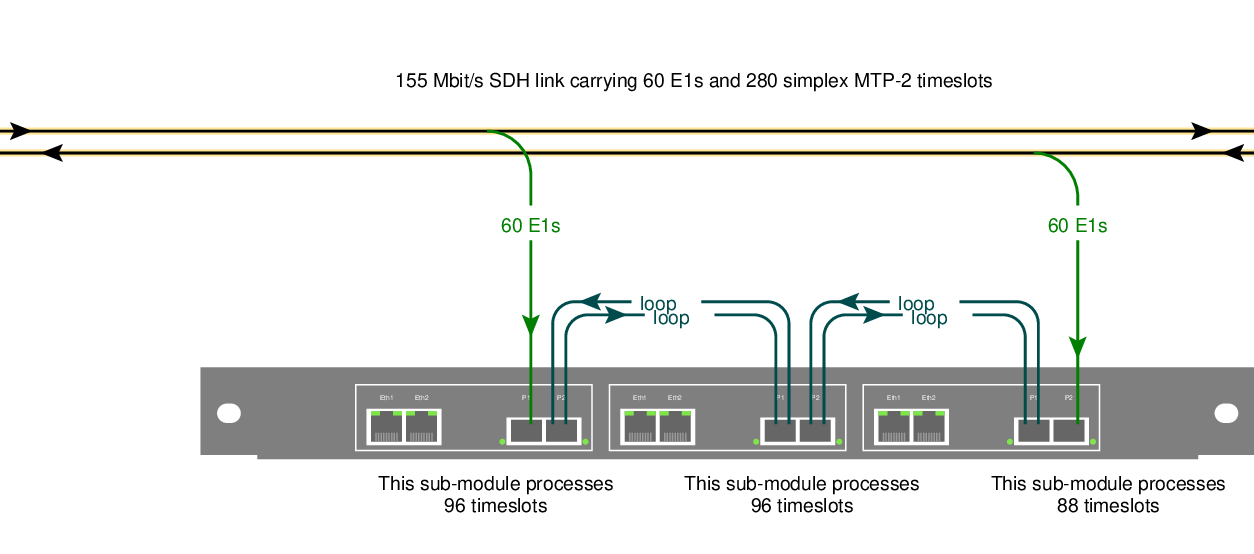
Ad-hoc daisy-chaining
An earlier post briefly mentioned daisy-chaining. We'll look at the same site: it has three SDH links, S1, S2 and S3. Each link is tapped with an optical splitter. It looks like this:
Each optical link in the example carries 10 LAPD timeslots per E1, that's fairly typical on Abis links. One STM-1, the one labelled 'S2', is fairly uninteresting because it only carries 300 channels of signalling:
15 E1s x 2 directions x 10 timeslots = 300 simplex channels
one submodule of an SDH/SONET Monitor 3.0 can decode all of that.
The STM-1 labelled 'S1', however, carries 500 channels of signalling, which is more than the 320 channels one submodule can decode:
25 E1s x 2 directions x 10 timeslots = 500 simplex channels
The solution is to re-transmit the incoming signal to another submodule. That's what the blue lines in the diagram show. We added a short fiber going from one sub-module to another. That lets us process 320 of the 500 channels on one submodule and 180 on the other.
Symmetric daisy-chaining
I called the daisy-chaining scheme above "ad-hoc", because it fairly arbitrarily copies some directions of some links to another submodule but leaves others alone. There's a second way to do daisy-chaining. Here's an example:
The idea is to feed each direction of a link into a separate submodule, and then copy both directions to a chain of submodules using short fiber cables. In this example, I've shown a chain of three subsubmodules.
Symmetric daisy-chaining lets every sub-module in the chain see all input. You can freely choose which sub-module in a chain processes which signalling channels---e.g. you might want to process the two directions of one signalling link on the same submodule.
The upside of symmetric daisy-chaining is that it's conceptually cleaner: every submodule in a chain sees all of the input.
The downside: symmetric daisy-chaining requires more fibers and in some situations also more hardware.
Intrusive monitoring
Normally, Corelatus hardware connects to optical networks via an optical tap. That way, you can be confident that the monitoring equipment won't disturb the live link.
With daisy-chaining, you also have the option of routing a live signal through the SDH/SONET monitor 3.0, i.e. you don't need an optical splitter. That's particularly useful in situations where briefly interrupting a link is acceptable, e.g. during a site survey or while debugging.
N.B.: daisy-chaining stops working when the power is off! That's why we use optical splitters for permanent installations.
How to set up daisy-chaining
Daisy-chaining always works cross-wise, i.e. a signal coming in on P1 (the leftmost SFP) will come out on P2. Daisy-chaining is off by default. Here's how to enable it:
    <enable name='sdh1'>
      <attribute name='daisy_chain' value='true'>
    </enable>
Here's what the same command looks like from the CLI:
    GTH CLI started. 'help' lists commands
    gth 172.16.1.34> enable sdh1 daisy_chain true
    ok
Permalink | Tags: GTH, telecom-signalling, SDH and SONET
Getting hex dumps of E1/T1 timeslots
Posted May 7th 2014
This post looks at a few simple tricks for understanding the WWW browser-based hex dump from a typical E1/T1 and then moves on to some more complicated things you can do with timeslot data by piping it to the standard (from BSD, but now on most unix-like systems) hexdump tool.
Browser-based hex dumps
The HTTP server built into GTH (and STH 3.0) lets you click your way to a timeslot-by-timeslot hexdump of an E1/T1. It shows 8ms of data, which gives you a rough idea of what's happening on an E1/T1:
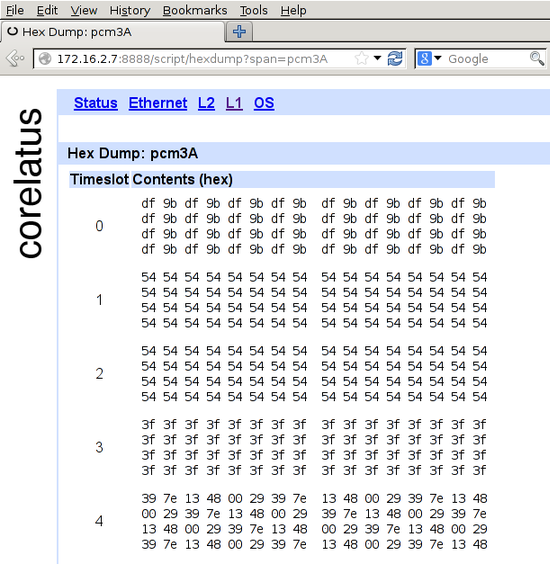
The HTTP server is on port 8888. To get to the hex dump, click 'L1' (at the top), then the E1/T1 you're interested in, for instance pcm4A, then 'hex dump' (at the bottom).
In the screenshot, timeslot 0 has a repeating two-octet pattern typical of an E1 link using doubleframe.
Timeslots 1 and 2 have the default idle pattern for E1 links: hex 54. That's silence, so those timeslots are most likely unused for the moment.
Timeslot 3 has nonstop 3f 3f 3f 3f. Writing that out in binary, 00111111001111110011111100111111, lets you see the pattern of six ones with a zero on either side. That's a flag. ISDN LAPD and Frame Relay links transmit flags between packets. Timeslot 3 probably contains LAPD signalling. There are eight possible bit rotations of the flag: 7e, e7, fc, cf, 9f, f9, 3f, f3.
Timeslot 4 has a repeating six-octet pattern. That's an MTP-2 FISU. Timeslot 4 is almost certainly running MTP-2.
Command-line hex dumps
This section assumes you're comfortable compiling C programs and using a Unix-like operating system, probably one of the BSDs or Linux. (You can do the same thing using Python, if you prefer, there's sample code for that too.)
Corelatus.com has some C sample code. It's also on github. Using that code, you can record a timeslot to a file:
./record 172.16.2.8 4A 1 /tmp/recording.raw
Let it run for 10 or 20 seconds, then stop it with ^C. You can now look at the data using the standard BSD tool 'hexdump' (on Debian, it's in the 'bsdmainutils' package):
tmp >hexdump -C recording.raw  | head -2
00000000  72 f9 d8 76 e5 df d6 fd  dc 5d ff f5 f0 94 57 da
00000010  eb 6e fa e4 7d 90 e4 e0  91 e2 eb ea ed e4 e3 e4
There's no limit to how large such recordings can be, so if you're debugging something, you can leave the recorder running for hours.
Live hex dumps
The 'record.c' sample code can also write to standard output. You can use that to get a live view of a timeslot via hexdump:
c >./record 172.16.2.7 3A 3 - 2>/dev/null | hexdump -C
00000000  3f 3f 3f 3f 3f 3f 3f 3f  3f 3f 3f 3f 3f 3f 3f 3f
*
The example above demonstrates a neat feature in 'hexdump': 'hexdump' suppresses repeated data. So you can leave it running in a window and it'll only produce output when something changes.
Permalink | Tags: GTH, telecom-signalling, C
save_to_pcap now supports PCap-NG for Wireshark
Posted December 15th 2013
Problem: you want to sniff packets from many SS7 signalling timeslots on many E1/T1s at the same time and analyse them with Wireshark.
Until now, the only way to know which packet came from where was to look at the DPC/OPC. Why? Because the PCap file format, used by Wireshark, tcpdump and many other tools, doesn't have any way to keep track of which interface a packet came from.
Solution: PCap-NG is a completely new file format which lets you keep track of which interface a packet came from. Wireshark understands PCap-NG (and, of course, classic PCap).
save_to_pcap
The C sample code from Corelatus includes a program called 'save_to_pcap' which takes SS7 packets from Corelatus E1/T1 and SDH/SONET hardware and translates them to PCap so that Wireshark can read them.
'save_to_pcap' now saves to PCap-NG by default. Wireshark 10.8 (released in June 2012) reads and writes PCap-NG by default. Here's how to capture packets from 8 signalling channels at the same time:
  $ ./save_to_pcap -n 8 172.16.2.8 1A 1B 2A 2B 16 2 load_generator.pcapng
  monitoring 1A:16
  monitoring 1B:16
  monitoring 2A:16
  monitoring 2B:16
  monitoring 1A:2
  monitoring 1B:2
  monitoring 2A:2
  monitoring 2B:2
  capturing packets, press ^C to abort
  saving to file load_generator.pcapng.1
  saving to file load_generator.pcapng.2
I used '-n 8' to force the capture file to rotate after 8 packets. That gives us clean, closed file to look at. Here's what it looks like in wireshark:
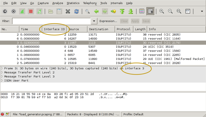
I've drawn yellow ellipses around the new parts. To get the "Interface ID" column:
- right-click on one of the existing column headings
- select "Column Preferences"
- select "Field type: Custom" and "Field name: frame.interface_id"
- Add
- OK
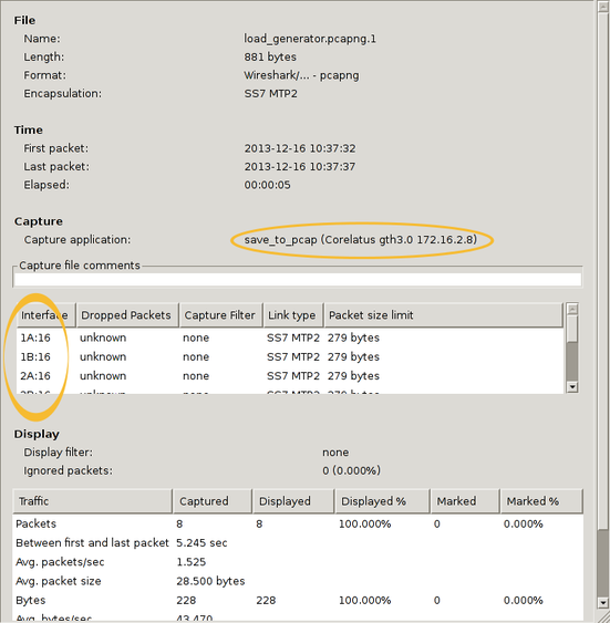
There's actually more information in the PCap-NG file. Wireshark shows it in the Statistics/Summary menu. This shows you the full interface names, i.e. "interface 1" is actually E1/T1 port 1B, timeslot 16 and you can also see exactly which GTH the capture came from.
You can also use 'frame.interface_id' in filter expressions.
PCap-NG is a nice format
The PCap-NG format is nicely designed, much better than the original PCap format. Had PCap-NG been around 13 years ago, we probably would have made GTH output traces directly in this format. It's flexible enough to let us include all sorts of information, e.g. we could even add layer 1 status changes on a separate "interface".
Wireshark limitations
PCap-NG is still relatively new in Wireshark, so there are few things that will probably improve with time. The ones I noticed are:
The 'if_name' field, i.e. the descriptive name for an interface, isn't available in the packet detail pane in the Wireshark gui. That means you just have to know that "interface 3" corresponds to, say, 4A:16. This was briefly discussed on the Wireshark mailing list, it looks like it'll eventually be added.(Edit 13. November 2014: done in Wireshark 1.12.1)- It looks like live captures in Pcap-NG format don't work. Wireshark just says "unknown format". You can work around that by reverting to the classic format, using the -c switch on save_to_pcap.
Getting the code
The C sample code is here and also on github.
Permalink | Tags: GTH, telecom-signalling, wireshark
Dimensioning SDH/SONET monitoring
Posted February 27th 2013
Updated 6. February 2018 because of capacity improvements in hardware shipped from this date onwards. This affects the LAPD capacity calculation.
This post is an example of how to figure out how much hardware you need to monitor all the Abis signalling at a GSM site which uses STM-1 to transport E1 lines.
The site
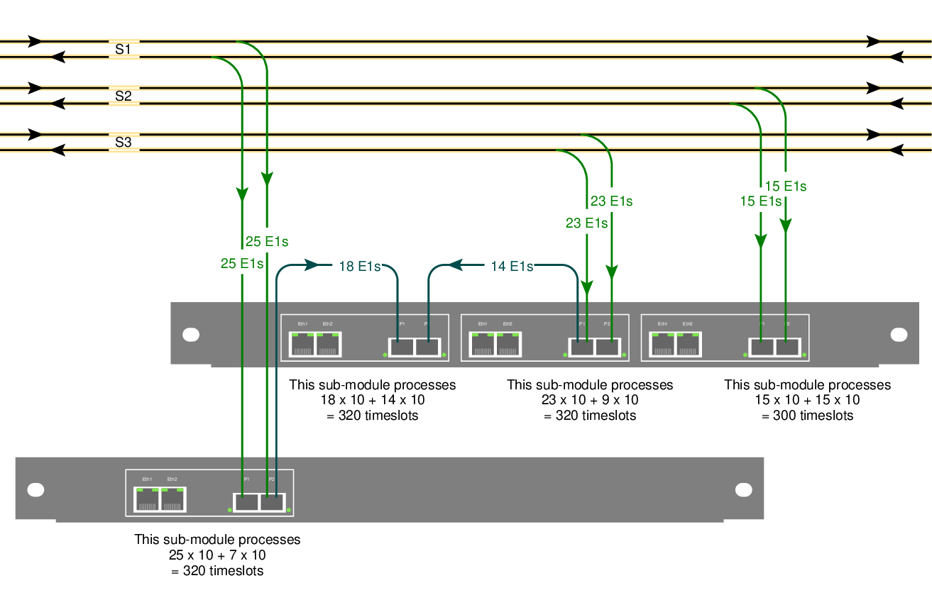
The site we're looking at, a BSC, has STM-1 connections to three BTSs: S1, S2 and S3. They have 25, 15 and 23 E1s on them. Here's how we set it up:
The yellow lines at the top are the original 155Mbit/s STM-1 links going from the BSC to each BTS. There's one fiber for each direction.
The green lines are the output of the fiber taps. They're an optical copy (typically taking 10% of the light) of the original STM-1. Each link has two taps, one for each direction. For this example, we'll assume that the application needs the signalling from both directions.
The blue lines are fibers going from one SDH/SONET probe's sub-module to another. That lets us shift processing load from one sub-module to another.
Ports and modules on Corelatus' SDH/SONET probe
There are two models of the SDH/SONET probe.
The lower one in the diagram is the low-end model: it has one sub-module. A sub-module has two SFP sockets and two ethernet ports. The SFP sockets accept SFP modules which connect to the optical lines (green).
The upper one in the diagram is the full model: it has three sub-modules.
Layer 2 (LAPD) signalling
For this example, I've assumed that we're interested in 10 timeslots of LAPD signalling on each E1. That's the worst-case in normal GSM installations. In practice, there can be fewer signalling timeslots, either because BTSs are daisy-chained or because the BTS doesn't have the maximum number of radio transceivers.
Each submodule can decode 400 LAPD channels. Link S1 has 25 x 2 x 10 = 500 LAPD channels, so one submodule can't process them all. We handle that by running a fiber to the next sub-module. That way, 25 + 7 E1s are handled on the first submodule and the remaining 18 on the next sub-module.
UMTS
On 3G networks, the signalling is often carried as ATM, either directly on STM-1 (or OC-3) or inside E1 lines carried on STM-1. The principles for dimensioning are the same, but the numbers are different.
Permalink | Tags: GTH, telecom-signalling, SDH and SONET
Configuring SDH/SONET
Posted January 30th 2013
Today, I'm going to walk through setting up a Corelatus SDH/SONET probe to look at E1/T1 lines carried on 155 Mbit/s SDH/SONET.
A quick look at SDH/SONET
Wikipedia has a good article about SDH/SONET. SONET is the standard mostly used in North America, SDH is the one mostly used in the rest of the world. The differences between the two are minor, for Corelatus' hardware it's just a setting in software.
SDH/SONET can both be used to carry various types of data. This time around, we'll just look at the E1/T1 lines. Here's a diagram of the scheme SONET uses to pack many E1/T1 lines into one 155 Mbit/s line, usually an optical fiber:
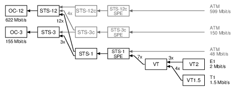
SONET calls the 155 Mbit/s line an "OC-3" (on the left of the diagram). SONET then has three layers of packing lines together (STS-1, VT, VT2), and that allows it to fit 3 x 7 x 3 = 63 E1 lines or 3 x 7 x 4 = 84 T1 lines.
SDH uses different names for similar ideas. The end result is the same: it carries 63 E1s or 84 T1s:
To work with E1/T1 lines on a Corelatus SDH/SONETs Monitoring Probe, we need to do three things:
- Turn on (enable) SDH/SONET at the top level
- Obtain (map) a name for a particular E1/T1 line
- Turn on (enable) layer 1 processing on the E1/T1 line
Setting up SDH/SONET using the API
Same as all other Corelatus probes, the SDH/SONET probe responds to text commands sent over TCP port 2089. To support SDH/SONET, we added two new comands enable and map.
First, enable SDH/SONET at the top level, in SONET mode for this example:
  C: <enable name='sdh1'><attribute name='SONET' value='true'/></enable>
  G: <ok/>
Once sdh1 is enabled, you can walk through the containers carried on it using the query command. But we'll skip right to mapping one of the E1 links:
    C: <map target_type='pcm_source'>
          <sdh_source name='sdh1:hop2:lop7_4'/></map>
    G: <pcm_source name='pcm60'/>
Now that we know what name the E1 has (pcm60 in this example), we can enable L1 using the same command you'd use on a probe with an electrical E1:
    C: <enable name='pcm60'><attribute name='mode' value='T1'/></enable>
    G: <ok/>
After these three commands, you have a T1 which is ready to use just like a T1 on other Corelatus hardware, i.e. you can start layer 2 decoding on it, or copy out the data or...
The API manual goes into detail, with more examples, including how to use disable and unmap.
Setting up SDH/SONET using the CLI
The SDH/SONET probe has a command-line interface. It's useful for experimenting and exploring. Here's how to set up things the same as above:
    $ ssh cli@172.16.2.9
    cli@172.16.2.9's password: (mail matthias@corelatus.se)
    GTH CLI, press Enter to start (^D to exit)

    GTH CLI started. 'help' lists commands
    gth 172.16.2.9> enable sdh1 SONET true
    ok
    gth 172.16.2.9> map sdh1:hop2:lop7_4
    Mapped to: pcm60
    ok
    gth 172.16.2.9> enable pcm60 mode T1
    ok
Setting up SDH/SONET using Python
Corelatus has sample code in a few languages, including Python, which shows how to use the API to set up an SDH link just like above. Here's the python demo program doing the same thing:
    $ ./gth.py enable 172.16.2.9 sdh1 SONET true
    $ ./gth.py map 172.16.2.9 sdh1:hop2:lop7_4
    pcm60
    $ ./gth.py enable 172.16.2.9 pcm60 mode T1
The C and Erlang sample code (on the same page) provides the same functionality, but with slightly different syntax.
Permalink | Tags: GTH, python, SDH and SONET
Retroactive debugging: recording signalling for later analysis
Posted December 6th 2012
This post is about saving signalling data for later analysis.
Problem: a subscriber reports that it wasn't possible to call a particular handset two hours ago. Connecting a signalling analyzer now won't help, so the best you can try to do is to reproduce the problem with test calls.
An alternative approach is to save all signalling data for a few days. Then, when you get a trouble report, examine the signalling affecting the subscriber's handset around the time the problem actually happened.
Disk space
Signalling on a single timeslot of an E1 cannot possibly be more than 8 kByte per second in each direction. There are 86400 seconds in a day and you usually save both directions of the link, so there's never going to be more than 140 MByte of data per day per ordinary link, uncompressed.
Real-world links aren't going to be anywhere near that busy. It's more likely that they're only carrying a few megabytes of signalling per day.
Even on high-speed-signalling-links at 1980 kbit/s, it's never going to be more than 5 GByte per day.
Sample code
The C sample code has an example which saves signalling from as many links as you want to a file in PCap format.
./save_to_pcap -m -n 1000 172.16.1.10 1A 2A 16 captured_packets.pcap
'-m' tells the GTH that the incoming signal is attenuated by 20dB
'-n 1000' means that you want a new '.pcap' file after every 1000 packets;
the files automatically get a .1, .2, .3, ... suffix.
'1A 2A' tells the GTH that you want packets captured on the E1/T1 interfaces called 1A and 2A.
'16' tells the GTH that you want timeslot 16
The PCap files can then be opened by wireshark, here's an example of doing that.
Permalink | Tags: GTH, telecom-signalling
Upgrading firmware on GTH
Posted May 31st 2012
This note is about two ways to upgrade the firmware on Corelatus hardware. For one-offs, you can use a browser-based upgrade. For large installations, it's easier and much faster to use a program which talks to the GTH's API on port 2089.
A Few Principles
All GTH hardware Corelatus has ever shipped (at the time of writing: GTH 1.x, GTH 2.x and the RAN probe) uses the same principles and methods for upgrading the firmware.
GTH has two completely separate firmware images. That way, things like a power failure in the middle of an upgrade, or a corrupt firmware image won't leave you with a 'bricked' system.
The two firmware images on the GTH are called system and failsafe. During everyday operation, the system image is used, it supports the full set of GTH commands. In exceptional circumstances, for instance while upgrading, the failsafe image is used. The failsafe image provides just enough functionality to support upgrading and troubleshooting.
The In-Browser Approach
- Get a firmware image from corelatus.com (mail matthias@corelatus.com to get a password)
- point your browser at the on-board serivce page: http://172.16.1.10:8888/service.html
- Select the 'Install firmware' link and follow instructions. The whole upgrade process will take two or three minutes.
catch-22: You can't use the browser-based upgrade systems running firmware from before May 2010, you need at least gth2_failsafe_10 and gth2_system_34a.
The API/Program Approach
For installations with tens or hundreds of modules, upgrading via a webbrowser is a waste of time. It's better to use the GTH's API on port 2089.
The quickest way to get started with that is to use Corelatus' sample code. We have working examples in
C: install_release.c, included in the C sample code.
Java: gth_upgrade.jar, included in the Java sample code.
What the API/Program Upgrade is Doing
The API-driven upgrade checks what firmware version is running, reboots the system to the 'failsafe' firmware, installs the release and checks that the installation succeeded. Breaking that down into steps:
Step 1: Check which image is running
Do that by issuing a query command
    <query>
    <resource name="system_image"/>
    </query>
The GTH replies with something like:
    <state>
    <resource name="system_image">
    <attribute name="version" value="development_release_9"/>
    <attribute name="locked" value="false"/>
    <attribute name="busy" value="true"/>
    </resource>
    </state>
You can tell that the GTH is running the system_image because busy=true. There are three circumstances under which the failsafe image may be booted:
- The system image is damaged, for instance as result of a failed upgrade.
- The GTH has attempted more than 5 consecutive boots without successfully booting. "Successfully booting" is defined as completing the boot process, starting the API and staying up for four minutes.
- The boot mode has been manually set to failsafe before the most recent boot.
Step 2: Boot the failsafe image
Images are not upgraded in-place, so if we want to upgrade the system image, we need to boot failsafe first. Do that by setting the failsafe boot mode
    <set name="os">
    <attribute name="boot mode" value="failsafe"/>
    </set>
and then sending a reset command:
    <reset>
    <resource name="cpu"/>
    </reset>
Step 3: Unlock the System Image
To make it a bit harder to accidentally upgrade a system, you have to 'unlock' an image before upgrading it:
  <set name="system_image">
  <attribute name="locked" value="false"/>
  </set>
Step 4: Install the new release
Upgrades to the image are standard compressed 'tar' archives.
Install them using the install command:
<install name="system_image"/>
The actual archive is sent immediately following the install command, in a block with content type 'binary/filesystem'.
The GTH sends an ok response after the filesystem has finished transferring. The actual install process continues after the transfer, an event is sent when it completes:
<event><info reason="install_done"/></event>
If you reboot without waiting for the install_done message, you'll probably get a corrupted installation. Start again from the top.
Step 5: Verify that the install completed
A query of the system image, as shown above, reveals the version number of the installed image. An install which has not completed shows up as empty.
Finally, we reboot again. If the system fails to boot after five attempts, the failsafe system starts.
Upgrading the Failsafe System
Upgrading the failsafe image is analogous to upgrading the system image. A special failsafe firmware release file is used.
Decoding signalling on the Abis interface with Wireshark
Posted February 25th 2012
Wireshark can decode the packets on GSM Abis links (and, probably also UMTS Iub). To do it, you need to first capture the data using a GTH, which is basically the same process as described in this entry about capturing data from the Gb interface, except for one difference: you want to capture LAPD, not Frame Relay:
save_to_pcap:lapd("172.16.2.7", "3A", 1, "abis.pcap").
Wireshark can open the file 'as is', but it only decodes up to L2. To get wireshark to decode everything, go to Edit/Preferences/Protocols/LAPD and then tick the "Use GSM SAPI values" checkbox. Presto, you get the RSL (Radio Signalling Link) protocol decoded for you. Nice.
Standards
The signalling protocol on GSM Abis links is specified in ETSI TS 100 595. ETSI specs are freely available from ETSI, you just have to register with an email address.
Permalink | Tags: GTH, telecom-signalling, wireshark
Controlling a GTH from Amazon EC2
Posted October 1st 2011
This post is about what I did to get the GTH example code (the C version) to run on Amazon EC2, controlling a GTH on the public internet.
Amazon EC2 is a service where you rent a virtual server by the second. The virtual server can run Windows or Linux. Our in-house environment is all-linux, so we use EC2 to give us an on-demand Windows environment to check example code on.
Overview
- Connect a GTH to the Internet
- Create and set up an Amazon EC2 Instance running Windows Server
- Install the example code
- Open up holes in the firewall
Taking each step in detail:
Connect a GTH to the Internet
First off: spend a moment thinking about security. You probably don't want SS7 traffic from a live network going over the internet. The GTH is designed to be installed in a secure network, not directly facing the internet. Take care.
Most likely, you've got the GTH behind a firewall. The firewall needs to be configured so that TCP port 2089 gets to the GTH.
The GTH needs to be told where the firewall is. In my case, it's at 172.16.1.1:
query_set 172.16.1.10 eth1 "default gateway" 172.16.1.1
Create an Amazon EC2 Instance
I'm assuming you're familiar with Amazon EC2. It's your choice which OS you want to run at Amazon. In my case, I wanted Windows because our primary development environment is linux, so I like the convenience of starting up an Amazon machine when I need to do something with Windows.
Install the example code
An easy way to do that is to use a WWW browser on EC2 to download the example code from corelatus.com.
On Amazon windows instances, an alternative is to use a remote share via terminal server. Still another is to install 'putty' and use 'psftp' to get the code from your own server.
Now you can try out the install:
> query_set 128.250.22.3 board
LED mode=normal
PCM LED assignment=universal
voice coding=alaw
architecture=gth2.1
ROM ID=0x26cbce800000005f
temperature=40.2
power consumption=6.4
power source=A
POE source=
'query_set' only uses the port 2089 API socket. But some of the other examples do more complicated things with TCP. 'playback_file', 'record' and 'save_to_pcap' all open TCP connections back to EC2 to send data.
Relaxing firewall rules
There are three places which are likely to block TCP connections originating at the GTH. You need to make sure each of those lets them through.
- The firewall between the GTH and the internet needs to allow the GTH to make outbound TCP connections. On most small firewall setups, that's the default. Some firewalls block outbound connections entirely, in which case you're out of luck (unless you can tunnel TCP through something else, such as SSH or an HTTP/1.1 proxy, but even that will require modifying the example code to use known port numbers).
- The firewall in EC2 Windows "security groups" needs to allow inbound TCP connections on all ports, as long as the originate from the GTH. Use the "Security Group" screen of the AWS console, in the "inbound" tab create a new rule. Use the internet-facing IP address the GTH has as the "source" IP. That way only the GTH can connect to your EC2 instance.
- Windows' own firewall needs to allow inbound TCP connections.
Either make a program-specific exception, or disable the windows
firewall entirely (and just rely on EC2's firewall).
netsh firewall add allowedprogram c:\users\mml\downloads\save_to_pcap.exe mode=ENABLE
All done
Now you can run use pretty much anything in the GTH API from a machine in Amazon's cloud.
Live Wireshark captures on Windows
Posted June 15th 2011
Update 23. January 2014: the -c switch is needed to force save_to_pcap to emit data in classic Pcap format, instead of Pcap-NG. Wireshark 1.10.5 doesn't allow Pcap-NG in pipes.
I've written about using Wireshark to look at signalling captured from an E1/T1 before. As of a few days ago, it's possible to do live captures on Windows, like this:
 save_to_pcap -c 172.16.1.10 1A 2A 16 \\.\pipe\ss7.1
 wireshark -k -i \\.\pipe\ss7.1
When you're capturing live, the SS7 packets appear in Wireshark in real-time.
The new version of 'save_to_pcap' program is part of the C examples, the .zip file contains both source (compiles on Unix and Windows) and .exe files.
It's always been possible to do live captures on Unix, you just pipe stdout:
./save_to_pcap -c gth21 1A 2A 16 - | wireshark -k -i -
Porting C socket code to Windows
Posted June 16th 2010
I just ported the C example code for controlling Corelatus E1/T1 hardware to Visual Studio 2010. Doing that was easier than expected. This first part of this post is about how to use that code. The second part is a bit of history about what I had to do to port the code.
Obtaining Visual Studio
Microsoft have their C/C++ compiler available for free download on microsoft.com
The install process is pretty standard for windows, if you're accustomed to Microsoft products, there are no surprises here.
Compiling the code
- Start the "Visual Studio Command Prompt". By default, that's in "Start/Programs/Microsoft Visual Studio 2010 Express".
- Navigate to the directory you unpacked the sample code in. Remove any old .exe files with 'del *.exe'.
- Run 'nmake /f NMakefile'. After a couple of seconds, you have six brand-new .exe files. Here's what this step looks like:
If you just wanted to see how to compile the code, you can stop reading now. The rest of the post is just about what I had to do to make this work with Microsoft's compiler.
Hurdle #1: MS nmake vs gnumake vs Visual Studio projects
Conclusion: I ended up using Microsoft's nmake and wrote a separate NMakefile for it.
My code gets built by 'make', through a Makefile. Visual Studio doesn't include a make program which can understand normal Makefiles, leaving me a choice of either using the Visual Studio IDE or using Microsoft's nmake.
I spent half an hour trying the IDE route. When you make a new project, you have to choose what sort it is. "CLR Console Application" seemed closest to what I wanted to do, so I chose that. Maybe "Makefile Project" would have worked better. Things got increasingly confusing from there. What's a "solution?" Why are "precompiled headers" enabled? I just want to compile a few hundred lines of C. At that point, I gave up, the IDE is clearly not the easiest way for me to get started.
Next, I tried Microsoft's replacement for make, called nmake. That didn't start flawlessly either, nmake uses its own syntax. Initially, I thought I might be able to write one Makefile which both gnumake and nmake understand. But Microsoft's syntax seems to be too different to allow that. Oh well. The NMakefile is just a dozen lines or so.
Hurdle #2: Missing header files
Conclusion: I used #ifdefs to include different header files when compiling in a win32 environment.
Visual Studio doesn't provide some of the header files the code uses, e.g. there's no 'unistd.h' and no 'sys/socket.h'. Odd. Providing most of unistd.h shouldn't be too hard.
The point of this exercise is to get the code to compile using a Microsoft toolchain, so I didn't investigate using cygwin or mingw.
In the end, it turns out that I wasn't using anything from 'unistd.h' which didn't get provided by something else in win32. 'socket.h' (and friends) was a bit harder, but it turns out that's provided by 'winsock2.h'.
Hurdle #3: 'Mostly compatible' socket API
Conclusion: winsock2 is different to the BSD socket API, but the differences can be worked around with just a few changes.
Sockets were invented on unix, so I assumed that other OSes would just copy the interface. But no, not on win32. There seem to be at least two attempts to make a socket API for windows, called 'winsock' and 'winsock2'. The first seems to be deprecated. The main problems I hit were:
- You can't use close() on a socket, you have to use closesocket()
- You can't use read() on a socket, you have to use recv()
- errno doesn't report socket errors, you have to call a special Windows Socket error reporting function.
None of those problems are hard to get around.
Hurdle #4: GNU and Microsoft can't agree on function names
Both GNU and Microsoft have replacements for some functions which are prone to security problems. If you use plain strcat() or strcpy, visual studio warns about security problems.
Disabling the warnings would be quick but feels like cheating. So I looked at the 'less insecure' alternatives. GNU call them strncat and strncpy whereas Microsoft call them strcat_s and strcpy_s. And the arguments are the same way around. It would have been nice if GNU and MS had solved this the same way, but no. Minor annoyance.
Hurdle #5: Structure packing pragmas
Conclusion: Both MS and GNU understand the #pragma pack(N) syntax, but only GNU understands the __attribute__((__packed__)) syntax.
A couple of the examples (save_to_pcap.c and record.c) use structures to encode or decode data defined by an external format. For instance, here's what the wire format of a 'Pcap' protocol capture file looks like:
      typedef struct {
        unsigned int magic;
        unsigned short major_version;
        unsigned short minor_version;
        unsigned int GMT_to_localtime;
        unsigned int sigfigs;
        unsigned int snaplen;
        unsigned int network;
      } PCAP_global_header;
We have to tell the compiler that spacing out the fields to get a certain alignment isn't allowed. The recommended GNU way to do that is to add __attribute__((__packed__)) after the structure. The recommended Microsoft way is to add #pragma pack(1) somewhere before the structure, and then remember to change the packing back again before hitting any code which is sensitive to performance.
Since this is just example code, we don't care about that last bit of performance, so we can just leave the packing at 1.
Aside: the structure above is a bit sloppy because just quietly assumes that an int is 32 bits and a short 16.
Hurdle #6: Windows firewall
Some of the example code opens TCP sockets for listening. By default, the windows firewall doesn't allow that. Just click "fine, ok, let me do this".
Unfortunately, that looks ugly for the user---the program will fail the first time you run it, and the pop-up box says "publisher unknown". Does anyone know how to improve on this? It'd be nice if the user could approve the publisher, i.e. me, once, and then every program works.
How long did the porting take?
A couple of days, including getting Visual Studio installed. That's for a few thousand lines of code with a bit of socket IO and file IO.
If I had to do it again, it'd take an afternoon or so.
Decoding UMTS (3G) interfaces with Wireshark
Posted May 24th 2010
Many 3G networks use ATM on their internal interfaces, e.g. on the Iub and Iu-PS interfaces. Those interfaces carry both control information (radio environment information, attach/detach messages, location updates) and also subscriber data, for instance IP traffic.
Wireshark understands how to decode those ATM interfaces. Here's an example of an interface sniffed by a GTH. The interface was carrying IP traffic over ATM on an E1 line.
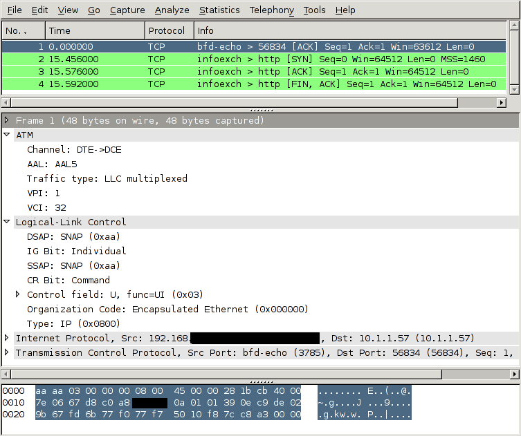
How to tell the GTH to capture an ATM link
To look at a 3G network like this, you need to:
- Connect one of the GTH's E1 interfaces to the E1 (or T1) interface carrying the ATM interface. You typically do that at a cross connect panel, using a G.772 monitor point.
- Enable the E1 interface you connected.
- Tell the GTH to start decoding ATM AAL5 (and/or AAL2) on that interface
- Convert the captured data to the file format which wireshark understands, libpcap.
- Open the captured file in wireshark. (It's also possible to pipe the captured data into wireshark live, both on Windows and Unix-like OSs).
Taking those steps one at a time, starting with #2:
Enable the E1 interface
<set name='pcm3A'><attribute name='monitoring' value='true'/></set>
Tell the GTH to start decoding ATM AAL5
IP traffic on ATM is always carried in AAL5. The timeslot arrangement is usually 1--15 + 17--31. A few sites share the E1 with other protocols, this is called fractional ATM. The GTH can handle either scheme.
  <new>
    <atm_aal5_monitor ip_addr='172.16.2.1' ip_port='1234' vpi='0' vci='5'>
      <pcm_source span='3A' timeslot='1'/>
      <pcm_source span='3A' timeslot='2'/>
      <pcm_source span='3A' timeslot='3'/>
      ..
      <pcm_source span='3A' timeslot='15'/>
      <pcm_source span='3A' timeslot='17'/>
      ..
      <pcm_source span='3A' timeslot='31'/>
    </fr_monitor>
  </new>
In this example, the VPI/VCI is 0/5. If you know the VPI/VCI in advance, great. If you don't, the GTH can sniff traffic at the AAL0 interface and show you which VPI/VCI are active on the link.
Convert the captured data
GTH sends out data in a format described in the API manual. Wireshark wants the data to be in libpcap format. save_to_pcap.erl, in the sample Erlang code for GTH can do the conversion, like this:
save_to_pcap:from_file("/tmp/captured.raw", "/tmp/captured.pcap").
A lazier approach is to let save_to_pcap.erl configure the GTH and start the capture:
  save_to_pcap:aal5("172.16.2.7", "3A", lists:seq(1,15) ++ lists:seq(17,31),
  {0,5}, "aal5.pcap").
The C version of save_to_pcap can currently only convert MTP-2, not AAL5. If you want it extended, send mail (address at top right).
Start up wireshark
Recent versions of Wireshark, e.g. 1.2.7, can decode such capture files out of the box, without any configuration. Finished.
Permalink | Tags: GTH, telecom-signalling, wireshark
Decoding the Gb Interface with Wireshark
Posted March 31st 2010
The Gb interface is part of the packet radio data network (GPRS) in GSM, it sits between the BSC and the SGSN and carries subscriber data headed to and from the internet.
Wireshark understands how to decode the Gb interface, so you can use wireshark to look through data sniffed from a Gb interface by a Corelatus GTH. Here's what it looks like:
How to tell the GTH to capture Gb
To look at a GPRS network like this, you need to do a few things:
- Connect one of the GTH's E1 interfaces to the E1 (or T1) interface carrying the Gb interfaces. You typically do that at a cross connect panel, using a G.772 monitor point.
- Enable the E1 interface you connected.
- Tell the GTH to start decoding frame relay on that interface
- Convert the captured data to the file format which wireshark understands, libpcap.
- Open the captured file in wireshark. (On unix-like operating systems, including OSX, you can also pipe into wireshark to get a live view of the capture.)
Taking those steps one at a time, starting with #2:
Enable the E1 interface
<set name='pcm3A'><attribute name='monitoring' value='true'/></set>
Tell the GTH to start decoding frame relay
The Gb interface uses frame relay on E1. Different sites use different configurations of timeslots. One common setup is to use timeslots 1--15. Another common setup is to 1--15 + 17--31. The GTH can handle any setup.
  <new>
    <fr_monitor ip_addr='172.16.2.1' ip_port='1234'>
      <pcm_source span='3A' timeslot='1'/>
      <pcm_source span='3A' timeslot='2'/>
      <pcm_source span='3A' timeslot='3'/>
      ..
      <pcm_source span='3A' timeslot='15'/>
    </fr_monitor>
  </new>
Convert the captured data
GTH sends out data in a format described in the API manual. Wireshark wants the data to be in libpcap format. save_to_pcap.erl, in the sample Erlang code for GTH can do the conversion, like this:
save_to_pcap:from_file("/tmp/captured.raw", "/tmp/captured.pcap").
A lazier approach is to let save_to_pcap.erl configure the GTH and start the capture:
save_to_pcap:frame_relay("172.16.2.7", "3A", lists:seq(1,15), "gprs.pcap").
The C version of save_to_pcap can currently only convert MTP-2, not frame relay. If you want it extended, send mail.
Start up wireshark
By default, wireshark decodes frame relay as 'FRF 3.2/CISCO HDLC'. That's not quite what we want. Go to Edit/Preferences/Protocols/FR and change the encapsulation to 'GPRS Network Service'. Now you get full decoding.
Permalink | Tags: GTH, telecom-signalling, wireshark
GTH 'C' API
Posted January 20th 2010
This post is for people who want to use C to control a GTH. Other languages (e.g. Erlang, Java, Python and Perl) are easier to work with, but in some applications you want the complete control that C gives you.
Corelatus provides a C API for GTH. The C API lets you control a GTH using plain C function calls---all of the XML wire format is taken care of.
Here's an example of how to use it to record speech on an E1/T1 timeslot, something you'd typically do in a voicemail system:
#include "gth_apilib.h"
...

  GTH_api api;                     // GTH_api represents one GTH API connection
  int result;
  int data_socket;
  char buffer[2000];
  char job_id[MAX_JOB_ID];
  int octet_count;

  result = gth_connect(&api, "172.16.1.10");    // Assuming the default GTH IP
  assert(result == 0);

  // We want to record audio on the E1/T1 called "1A", on timeslot 3.
  data_socket = gth_new_recorder(api, "1A", 3, job_id);

  while ( (octet_count = recv(data_socket, buffer, sizeof buffer, 0)) ) {
    // do whatever you want with the received data
  }

...
The recording above happens in the 'while' loop. It continues forever (i.e. until you abort it). The audio data is bit-for-bit identical to what was on the E1/T1 timeslot, so this can be used for recording both voice and signalling.
Further examples
The C API code includes further examples to:
- Record audio or signalling from a timeslot to a .wav file
- Play back previously recorded files
- Install (upgrade) the firmware on a GTH
- Monitor (sniff) SS7 MTP-2 and save the signalling to a wireshark (PCap) compatible file.
- Monitor CAS R2 signalling.
Standalone Parser
Aside: the C API code includes a standalone parser for the XML responses the GTH emits. You can use the parser without using the rest of the API library, if you want to.
Audio power levels on E1/T1 timeslots: the digital milliwatt
Posted October 10th 2009
Sometimes, you want to know when the audio on an E1/T1 timeslot has gotten louder than some limit. In a voice mail application, that's useful for catching mistakes such as a subscriber leaving a message but then not hanging up the phone properly—you don't want to record hours and hours of silence. In an IVR application, you might want to keep an eye on the audio level so that a frustrated (shouting!) subscriber can be forwarded to a human operator.
GTH provides a "level detector" to do that sort of thing. You start a level detector on a timeslot, give it a loudness threshold, and it'll notify you whenever the audio on the timeslot goes over that threshold. Here's an example command which notifies you if the power on timeslot 13 of an E1/T1 is louder than -20dBm0:
  <new><level_detector threshold='-20'>
     <pcm_source span='2A' timeslot='13'/>
  </level_detector></new>
The algorithm is:
- Take a 100ms block of audio (800 samples)
- Square all the samples
- Sum the squares
- If the sum exceeds the loudness threshold, send an XML event
There are some details to worry about.
The digital milliwatt
The threshold, e.g. -20 in the example above, has to be relative to something. The standard reference power level in telecommunications is the milliwatt. ITU-T G.711, table 5 and 6 defines the sequences which represent a milliwatt:
A-law: 34 21 21 34 b4 a1 a1 b4
μ-law: 1e 0b 0b 1e 9e 8b 8b 9e
Here's what a few periods of the digital milliwatt look like:

In this post, the unit 'dBm0' means power, in dB relative to the digital milliwatt, as defined by the sequences above. If you have no idea what dB means, wikipedia has a decent article.
What's the loudest possible sound on a timeslot?
170 is the highest value possible in A-law encoding. It corresponds to linear 4032. That's about 6dB louder than the digital milliwatt.
85 is the smallest value possible in A-law encoding. It corresponds to linear -1. That's about 66dB softer than the digital milliwatt.
The range -66dBm0...+6dBm0 sets an upper bound on the range of power on a timeslot. Then there are other things which further limit the practical range, so you're unlikely to actually use a +6dBm0 threshold in practice, but it's there if you want it.
Is the G.711 definition the best one?
The sequence given in G.711 is a 1kHz sine wave. The sampling rate on E1/T1 is 8kHz, so the reference sequence can be expressed in just eight values. That's nice, but that also leads to small errors, about 0.13dB, because of quantisation.
ITU-T O.133 discusses that problem in detail and proposes a test signal which specfically is not 1kHz (i.e. not a submultiple of the sampling rate). For most practical purposes, 0.13dB doesn't matter and so the simple and robust thing to do is to use the well-defined and well-known G.711 sequence as a reference.
Here's what a few periods of a 1020Hz signal look like. Notice that the samples, i.e. the red crosses, don't appear in the same spot one period later---that way we don't get the same errors over and over again.
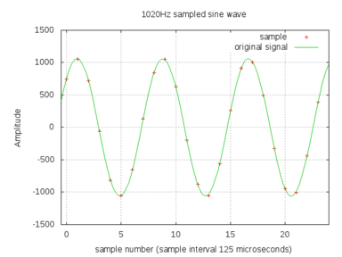
Testing pitfall: the .wav header
GTH players plays raw A-law or μ-law data. If you feed a player a .wav file in 8kHz A-law, or μ-law if your network uses μ-law, there will be a very short bit of noise at the start of the playback because the .wav header gets treated as though it were audio.
When testing level detection, especially at quiet levels, that header noise is enough to trigger a detector. Here's a .wav of a 1000Hz sine wave at about -30dBm0:
00000000  52 49 46 46 42 27 00 00  57 41 56 45 66 6d 74 20  |RIFFB'..WAVEfmt |
00000010  12 00 00 00 06 00 01 00  40 1f 00 00 40 1f 00 00  |........@...@...|
00000020  01 00 08 00 00 00 66 61  63 74 04 00 00 00 10 27  |......fact.....'|
00000030  00 00 64 61 74 61 10 27  00 00 d5 c4 f5 f1 f3 f1  |..data.'........|
00000040  f5 c4 d5 44 75 71 73 71  75 44 d5 c4 f5 f1 f3 f1  |...DuqsquD......|
*
00002740  f5 c4 d5 44 75 71 73 71  75 44                    |...DuqsquD|
The first 58 octets (bytes) are the header. If we turn that header into a periodic signal, it's at about -8dBm0, which is fairly loud. With the default period parameter of 100ms in the level detector, that'll cause a false level of about -11dBm0.
The period parameter
The level_detector has an optional parameter, the period. The period sets the size of the audio block the GTH considers when measuring the power. A short period makes the GTH responsive to sudden changes in power on the timeslot, which would be useful in an application such as figuring out which of the people in a conference call are currently talking. A long period averages out the power over a longer time, which is useful in deciding whether a voicemail recording has finished.
The default is 100ms.
Sample files
This .zip file contains sample recordings with 1kHz sine waves at 0, -10, -20, -30, -40 and -50 dBm0. The .wav versions are useful for listening to or importing into an audio editing program to calibrate the level meter. The .raw versions are just plain A-law samples---you can use them with a GTH player.
Permalink | Tags: GTH, telecom-signalling
How does TCP behave on an interrupted network?
Posted August 27th 2009
GTH E1/T1 modules are always controlled by a general-purpose server, usually some sort of unix machine. The server and GTH are connected by ethernet and communicate using TCP sockets. Normally, that ethernet connection is chosen to be simple and reliable, for instance by putting the server and the GTH in the same rack, connected to the same ethernet switch.
I experimented a bit to see what happens when that network gets interrupted. I interrupted the network in a reproduceable way by disabling and re-enabling the server's ethernet port for a known length of time while running a <recorder>. (A <recorder> sends all the data, typically someone talking, from an E1 timeslot to the server over a TCP socket, 8000 octets per second.)
Capturing the ethernet packets
Here's what I did to capture traffic and interrupt the ethernet:
  tcpdump -w /tmp/capture.pcap -s 0 not port 22
  sudo ifconfig eth0 down; sleep 5; sudo ifconfig eth0 up
A trace where traffic recovers in time to prevent an overrun
The GTH buffers about two seconds of timeslot traffic. So a 'sleep' of about a second won't result in an overrun. Here's what it looks like in wireshark:
| Packet | Time | Direction | Flags | Seq. # |
| 133 | 7.596 | GTH -> server | [PSH, ACK] | 59393 |
| 134 | 7.633 | server -> GTH | [ACK] | 1 |
| 135 | 7.724 | GTH -> server | [PSH, ACK] | 60417 |
| 136 | 7.761 | server -> GTH | [ACK] | 1 |
| 137 | 7.852 | GTH -> server | [PSH, ACK] | 61441 |
| 138 | 7.889 | server -> GTH | [ACK] | 1 |
| 139 | 7.980 | GTH -> server | [PSH, ACK] | 62465 |
| 140 | 8.017 | server -> GTH | [ACK] | 1 |
| 141 | 8.108 | GTH -> server | [PSH, ACK] | 63489 |
| 142 | 8.145 | server -> GTH | [ACK] | 1 |
| 143 | 8.236 | GTH -> server | [PSH, ACK] | 64513 |
| 144 | 8.273 | server -> GTH | [ACK] | 1 |
| 145 | 8.364 | GTH -> server | [PSH, ACK] | 65537 |
| 146 | 8.401 | server -> GTH | [ACK] | 1 |
| 147 | 10.151 | GTH -> server | [PSH, ACK] | 66561 |
| 148 | 10.151 | server -> GTH | [ACK] | 1 |
| 149 | 10.151 | GTH -> server | [ACK] | 67585 |
| 150 | 10.151 | server -> GTH | [ACK] | 1 |
Everything up to packet 146 is normal: the GTH (172.16.2.5) sends 8000 octets every second and the server (172.16.2.1) acks them. It happens to be in chunks of 1024 octets about eight times per second. After packet 146, about 8.4 seconds after the capture started, the ethernet interface went down and stayed down for 1s. The TCP stream started up again after about 1.5s and then 'caught up' by sending many packets in quick succession.
A trace where traffic didn't recover
I took a second trace similar to the first one, except this time, I disabled ethernet for about five seconds:
Packet Time     Source IP     Dest IP    SPort   DPort
----------------------------------------------------------------------
 28   1.040083  172.16.2.5 -> 172.16.2.1 54271 > 45195 [PSH, ACK] Seq=7169
 29   1.040095  172.16.2.1 -> 172.16.2.5 45195 > 54271 [ACK] Seq=1
 30   1.168065  172.16.2.5 -> 172.16.2.1 54271 > 45195 [PSH, ACK] Seq=8193
 31   1.168078  172.16.2.1 -> 172.16.2.5 45195 > 54271 [ACK] Seq=1
 32   1.296067  172.16.2.5 -> 172.16.2.1 54271 > 45195 [PSH, ACK] Seq=9217
 33   1.296079  172.16.2.1 -> 172.16.2.5 45195 > 54271 [ACK] Seq=1
 34   1.424068  172.16.2.5 -> 172.16.2.1 54271 > 45195 [PSH, ACK] Seq=10241
 35   1.424081  172.16.2.1 -> 172.16.2.5 45195 > 54271 [ACK] Seq=1
 36   7.782851  172.16.2.5 -> 172.16.2.1 54271 > 45195 [PSH, ACK] Seq=11265
 37   7.782863  172.16.2.1 -> 172.16.2.5 45195 > 54271 [ACK] Seq=1
 38   7.783406  172.16.2.5 -> 172.16.2.1 54271 > 45195 [ACK] Seq=12289
 39   7.783413  172.16.2.1 -> 172.16.2.5 45195 > 54271 [ACK] Seq=1
 40   7.783569  172.16.2.5 -> 172.16.2.1 54271 > 45195 [ACK] Seq=13737
...
 50   7.784962  172.16.2.5 -> 172.16.2.1 54271 > 45195 [FIN, PSH, ACK] Seq=23873
 51   7.784972  172.16.2.1 -> 172.16.2.5 45195 > 54271 [ACK] Seq=1
 52   7.785026  172.16.2.1 -> 172.16.2.5 45195 > 54271 [FIN, ACK] Seq=1
 53   7.785348  172.16.2.5 -> 172.16.2.1 54271 > 45195 [ACK] Seq=25322
Everything is normal up to packet 35. Then, ethernet is suspended for five seconds and TCP takes a further second to recover, which causes a buffer overrun on the GTH (172.16.2.5). The GTH closes the socket at packet 50 and also sends an overrun event to the application so that it knows why the socket was closed.
Bottom line
GTH uses IP for control and traffic. It is important that the IP link between the GTH and the server is simple and reliable. Ideally the GTH and server should be in the same rack and be connected by an ethernet switch.
It's possible for a system to survive a short interruption (less than a second) to the ethernet traffic without pre-recorded calls getting interrupted. For longer interruptions, all bets are off.
(Interruptions aren't the only type of network problem, e.g. radio networks such as 802.11 can suffer significant packet loss, which can trigger TCP congestion avoidance. But that's another topic.)
Permalink | Tags: GTH, questions-from-customers
Capturing SS7 with wireshark or tshark
Posted August 10th 2009
Update 23. January 2014: save_to_pcap now emits Pcap-NG by default, but current versions (1.10.5) of Wireshark don't allow that through pipes. Use the '-c' switch to force classic Pcap.
I often use wireshark to look at SS7 signalling on E1 links. Up until today, I've always done that by capturing the signalling (from a GTH), then converting the captured data to libpcap format and finally loading the file into wireshark.
Someone showed me a better way today: wireshark can read from a pipe or from standard input. That lets me see and filter the packets in wireshark in real time. Here's how to do it, using the save_to_pcap demo program (included in gth_c_examples):
> ./save_to_pcap -c gth21 1A 2A 16 - | wireshark -k -i -
capturing packets, press ^C to abort
saving capture to stdout
The same thing works for tshark:
 >./save_to_pcap -c gth21 1A 2A 16 - | tshark -V -i -
capturing packets, press ^C to abort
saving capture to stdout
Capturing on -
Frame 1 (15 bytes on wire, 15 bytes captured)
    Arrival Time: Aug 10, 2009 20:38:29.388000000
...
   Message Transfer Part Level 2
    .000 1101 = Backward sequence number: 13
    1... .... = Backward indicator bit: 1
    .011 1000 = Forward sequence number: 56
    1... .... = Forward indicator bit: 1
    ..00 0000 = Length Indicator: 0
    00.. .... = Spare: 0
...
Works on *nix and Windows
Piping standard output to wireshark/tshark works on all the *nixes, i.e. linux, BSD, OSX, Solaris. On Windows, things are a bit different, you have to use 'named pipes' instead, like this:
 save_to_pcap -c 172.16.1.10 1A 2A 16 \\.\pipe\ss7.1
 wireshark -k -i \\.\pipe\ss7.1
On some older (as of August 2009) versions of wireshark, possibly in combination with older libraries, the "-i -" switch doesn't work, at least according to google, even though the tshark version works.
Generating DTMF using a 'player' on GTH
Posted June 9th 2009
The GTH can transmit in-band signalling tones on a timeslot. That's useful for testing and for building active in-band signalling systems.
DTMF
The tones transmitted when the subscriber presses a number key on fixed or mobile handset are called DTMF. Wikipedia has an article about it. To generate DTMF, all we really need to know is that there are 16 possible DTMF signals, that each signal is made up of two sine waves of particular frequencies and that sending the signal for 100ms is a reasonable thing to do.
Here's a .zip file with DTMF tones in it. Each file is raw ALAW data, i.e. it's ready for the GTH to play (transmit) on a timeslot.
The GTH has two ways of playing tones. One way is to stream the audio data in over a TCP socket each time we want to play it. I wrote a post about that earlier. The other way is to store the sample data on the GTH and command its playback whenever it's needed. Since there's a small number of different tones (12, or 16 if you want to use the A/B/C/D tones as well) and the tones are short, storing them on the GTH makes sense. To store the tone:
<new><clip name='dtmf5'></new>
(and now send the 800 byte file)
to play the tone later on:
<new><player>
  <clip id='clip dtmf5'/>
  <pcm_sink span='3A' timeslot='19'/>
</player></new>
Sequences of tones
Sometimes you want to transmit a sequence of DTMF tones, for instance to simulate a subscriber dialling a number. The GTH lets you start a player with a sequence of tones like this:
<new><player>
   <clip id='clip dtmf5'/><clip id='clip dtmf6'/><clip id='clip dtmf8'/>
   <pcm_sink span='3A' timeslot='19'/>
</player></new>
But that isn't a valid sequence of DTMF tones. Why not? Because DTMF expects a gap between tones. The cleanest way to handle that is to define another clip consisting of just silence and putting it between each tone. A good 'silence' value on E1 lines is 0x54. 60ms (480 samples) is a reasonable length.
Other in-band tones
DTMF in-band signalling is used in pretty much all handsets (telephones), mostly for dialling, but also to navigate menus in IVR systems. But before SS7 became popular, in-band signalling in the form of CAS and SS5 was even used to communicate call setup information between exchanges. GTH can also generate those tones, but that can be the subject of another post.
Perl example code for GTH: SS7 ISUP decoding and playback/record
Posted May 28th 2009
To help people get started, www.corelatus.com has some example code for doing useful things with GTH units.
Now it also has Perl example code. It does the same thing as the python examples:
- Enable an E1/T1 port
- Start MTP-2 monitoring on a timeslot and decode SS7 ISUP (to print out when calls start and stop). I wrote a post a while back about how to decode ISUP.
- Dump the contents of a timeslot to a file (for later analysis)
- Feed a file into a timeslot (for playback of previously captured files)
It's built on top of a Perl module which provides a Perl API for a subset of the GTH API.
A quick example
Here's a quick example of how it's used. We want to enable (turn on) the first E1/T1 interface on a GTH module:
my $api = gth_control->new($host);
$api->send("<set name='pcm$span'><attribute name='mode' value='E1'/></set>");
defined $api->next_non_event()->{ok} || die("error from GTH (bogus PCM?)");
$api->bye();
It's good for experimenting.
The Perl module the examples are based on, gth_control.pm, is at a level which makes it useful for experiments and prototypes. To build a full-fledged product on top of it, more work is needed.
For a start, you'd probably want to move the XML generation (like the '<set name=...' code above) out of the application code and into the gth_control.pm module, thus making it a pure Perl interface.
Next, you need to come up with a strategy to deal with concurrency, because being limited to recording one timeslot at a time is fine for lab work, but not fine for (say) a voicemail system.
Download
The zipfile of the code is linked from the bottom of the API page.
Decoding MTP-3 and ISUP
Posted March 25th 2009
Sometimes, you want to look at the signalling on an E1 and use it to figure out when telephone calls start and stop. In SS7 networks, call setup and tear-down is done by the ISUP layer, which fits in to the SS7 stack like this:
Layer 4: ISUP
Layer 3: MTP-3
Layer 2: MTP-2
Layer 1: MTP-1 (typically an 2Mbit/s E1 or a 1.5Mbit/s/T1)
If you have a GTH connected to the E1 you're interested in, either via a DXC or a monitor point, the GTH takes care of layers one and two. That leaves MTP-3 and ISUP to you.
The easiest way to decode MTP-3 and ISUP is to let wireshark do it for you. There's a note about how to do that on Corelatus' official site. But this blog entry is about how to decode MTP-3 and ISUP yourself.
A signal unit (packet)
In SS7, packets are usually called "signal units". Here's what an SS7 signal unit looks like 'on the wire', octet by octet, with MTP-2 and MTP-1 already decoded:
  8d c8 1f 85 02 40 00 00  35 00 01 00 21 00 0a 02
  02 08 06 01 10 12 52 55  21 0a 06 07 01 11 13 53
  55 00 6e 00
MTP-3
The start of the packet is the MTP-2 (ITU-T Q.703) and MTP-3 (ITU-T Q.704) headers. These headers are easy to decode because they are always fixed-length:
| Octet(s) | Value | Purpose |
|---|---|---|
| 00--01 | 8d c8 | MTP-2 sequence numbers, safe to ignore |
| 02 | 1f | MTP-2 length indicator. Anything less than 3 is reserved for MTP-2 itself and should be discarded. |
| 03 | 85 | MTP-2 SIO. The SIO tells us which 'service' the signal unit is intended for. Q.704 sections14.2.1 and 14.2.2 tell us that anything ending in hex 5 is for ISUP. |
| 04--07 | 02 40 00 00 | MTP-3 Routing label. The routing label is just a "from" and "to" address in the SS7 network. For most applications we can ignore it. Q.704 figure 3 shows what's in the routing label. |
Upshot: to see calls start and stop, all we have to do for MTP-3 is:
- Look at the length indicator (offset 2) and discard any signal unit where it's less than 3.
- Look at the SIO (offset 3). Discard if (SIO & 0x0f != 5)
ISUP
The rest of the signal unit is ISUP. Annex C in ITU-T Q.767 tells us how to decode ISUP. ISUP is fiddly because there are several types of ISUP packets, because several of those types have optional fields and because some of those fields are variable length. Here are the octets we have left after removing MTP-2 and MTP-3:
  35 00 01 00 21 00 0a 02
  02 08 06 01 10 12 52 55
  21 0a 06 07 01 11 13 53
  55 00 6e 00
The first two octets are the CIC. The third octet is the Message type.
The CIC (Q.767 C.1.2) tells us which circuit this call uses. All the signalling for one call has the same CIC. In ITU networks, it's a 12-bit value packed into the field in little-endian byte order. In this case CIC=0x0035. We're sniffing an E1 line, so C.1.2.a tells us that the lower five bits correspond to the timeslot (timeslot 5) and the rest identifies the E1 itself.
The Message Type (Q.767 Table C-3) field tells us what sort of ISUP message this signal unit is. 0x01 is an IAM. 0x10 is RLC. For a minimal "show me what calls are going through the system" hack, we only need to look at the IAM (comes at the start of the call, contains the A and B numbers) and the RLC (sent when the call is finished) messages.
Now we know that the CIC=0x35, that the message is an IAM and we still have about a dozen octets to decode. Q.767 table C-16 tells us how to decode an IAM. There are some uninteresting fixed-length fields followed by the B number and then the A number. Look at the code (or Q.767, section C.3.7) if you're interested in the details. All we really care about is that these octets
06 01 10 12 52 55 21
represent the B number: 21255512. You can see the number in the raw data if you skip the first three octets and swap every second digit.
Turning those ISUP steps into an algorithm to decode one signal unit:
- Save the CIC
- Is the message an IAM? Decode it as an IAM, which is fiddly.
- Is the message an RLC? Just print the CIC.
That's all you need to do to make a simple system which prints the start and end of each call. To do something useful, you need to maintain a table of in-progress calls and match up the IAM and RLC messages with the same CIC. You also need to handle things like systems restarting.
Further reading
The ITU now have most of their standards freely available at www.itu.int. So one way to learn more about MTP-3 and ISUP is to read the standards, e.g. all the Q-series standards about signalling are here.
Erlang code
Everything discussed above is implemented in the ss7_sniffer.erl example. It makes good use of Erlang's binary syntax, e.g. here's the MTP-3 decoder:
    mtp3(<<_Sub:4, Service_indicator:4>>, <<DPC:14, OPC:14, SLS:4,
						    Rest/binary>>) ->
	case Service_indicator of
	0 -> % Management
        ignore;
	1 -> % Test/maintenance
        ignore;
	3 -> % SCCP
        ignore;
	5 ->
        isup(DPC, OPC, SLS, Rest);
	9 -> % B-ISUP; similar to ISUP, but not compatible.
        ignore;
	X ->
        io:fwrite("ignoring SU with unexpected service indicator=~p\n", [X])
	end.
It looks a lot like one of the examples in the original paper about the binary syntax.
Python Code
The same thing done in Python is fairly straightforward once you discover the Python 'struct' library, which is basically the same thing as PERL's pack/unpack. The code is in sniff_isup.py, inside the GTH python examples zip.
Permalink | Tags: erlang, GTH, telecom-signalling, python
The timestamp field in signalling headers
Posted March 23rd 2009
When the Corelatus GTH is used to monitor (sniff) signalling, it sends each sniffed packet to your server over a TCP socket, along with a header. For instance, for SS7 MTP-2 the header looks like this:
octet 0x00: Length (16 bits) octet 0x02: Tag (16 bits) octet 0x04: Flags (16 bits) octet 0x06: Timestamp (48 bits)
Every field is big-endian, i.e. the most significant byte comes first. Here's an actual header from a GTH, octet by octet:
00 1c 00 00 00 00 01 20 34 ee fa 61 99 99 99 99 ...
The timestamp is thus 0x012034eefa61, or decimal 1237838658145. For most applications, you just want to know which packet came first, so the interpretation of that number doesn't matter much, though it's useful to know that it's the number of milliseconds since the unix epoch. (wikipedia has a decent article about unix time)
Sometimes, though, you want to represent that as a human-readable time. Unix (and, most likely, Win32) provides functions to do that in the C library, so, after throwing away the last three digits (the milliseconds), this C program does it:
#include <time.h>
#include <stdio.h>
int main() {
const time_t time_stamp = 1237838658;
printf("%d corresponds to %s\n", time_stamp, ctime(&time_stamp));
return 0;
}
The output agrees with what the clock on my wall says:
1237838658 corresponds to Mon Mar 23 21:04:18 2009
Python
Since I've been messing around with python, the same thing in python:
>>> import time >>> time.ctime(1237838658) 'Mon Mar 23 21:04:18 2009'
Erlang
Erlang doesn't have an interface to the 'ctime' call, but you can use the gregorian calendar functions:
1> Epoch = calendar:datetime_to_gregorian_seconds({{1970, 1, 1}, {0,0,0}}).
62167219200
2> calendar:gregorian_seconds_to_datetime(1237838658 + Epoch).
{{2009,3,23},{20,4,18}}
Why use milliseconds?
Why is the GTH timestamp in milliseconds instead of either seconds or a 'timeval'-like seconds + microseconds?
We chose millisecond resolution for several reasons. Firstly, the shortest possible useful packet in SS7 takes a bit more than a millisecond to transmit at 64kbit/s. Secondly, the practical limit of NTP time synchronisation over the internet is about one millisecond at a typical site.
GTH audio streaming: why stream over TCP?
Posted March 6th 2009
GTH lets you stream audio from a TCP socket to a timeslot on an E1/T1 line. Some people are surprised by the choice to use TCP. When I added that support back in 2002, my first thought was to use RTP (RFC 1889). RTP is simple: you just dump the audio in a UDP packet with some timestamping information and shoot it out on ethernet at the right rate.
I'd worked with RTP before and I'd been at a couple of SIP interops where most of the attendees had trouble emitting audio at 'the right rate', i.e. 8000 samples/s. One manufacturer's system would emit 8007 samples/s. Another would play it back at 7999 samples/s. What do you do with the extra 8 samples per second? If you do nothing, you get endlessly growing delays and, eventually, a buffer overflow. If you come up with a strategy for throwing away samples, it's bound to interact badly with something, sooner or later.
The thing is, when you're streaming in pre-recorded audio, you don't need it to be at the right rate. You just need to make sure it doesn't overrun or underrun the GTH's internal buffer. I.e. you need flow control, not rate control. TCP has flow control, and everyone knows how to use TCP sockets. In 2002, doing things that way was right at the limit of what our 50MHz embedded CPU could keep up with. Now it's no problem at all.
Python
I'm playing around with python at the moment. Here's how to put some data on an E1 timeslot, straight from the python shell. First, set up a listening TCP socket:
import socket s = socket.socket(socket.AF_INET, socket.SOCK_STREAM) s.listen(0) addr, port = s.getsockname()
Next, open another socket to the GTH command port (2089) and tell it we want to stream in audio on the socket we opened above:
a = socket.socket(socket.AF_INET, socket.SOCK_STREAM)
a.connect(("172.16.2.7", 2089))
my_ip, _port = a.getsockname()
command = "" % (my_ip, port)
header = "Content-type: text/xml\r\nContent-length: %d\r\n\r\n" % len(command)
a.sendall(header + command)
Finally, accept() and send the data:
d, _ = s.accept()
d.sendall("hello world")
d.close()
That looks OK to me, though I imagine the style betrays my Erlang mindset. There's a more complete python example at the bottom of the API page.
SOX parameters for downsampling to 8kHz Alaw
Posted February 19th 2009
A technician working for an operator mailed me a few days ago wondering why the recorded voice clips they use for their IVR sound so bad, "like they're coming from the bottom of a deep well". It turned out that the clips actually sounded OK on a telephone, just not through his laptop's speaker. He asked if I recommend any specific filter parameters when converting audio from 44.1kHz wav to 8kHz Alaw voice clips.
An example
I took this audio snippet from the introduction to an audio book. It was originally a .mp3 file. I converted it to a .wav file with a 44.1kHz sampling rate and 16 bits per sample. For my purposes, artefacts from mp3 are negligible.
Next, I converted it to 8kHz Alaw using sox. 8kHz Alaw is what runs on the fixed telephone network in most of the world. (The US uses a minor variant, μlaw):
sox 1_mono.wav --encoding a-law --rate 8000 2_8kHz_alaw.wav
That sounds a bit less clear than the original, but it's OK. It's what you'd expect coming out of a telephone. There's some weirdness though. The audible difference between the two files varies from one PC to another and even one playback program to another. Why? Because laptop speakers vary in quality and because playback programs usually quietly convert everything back to 48kHz or 44.1kHz sampling rates, and they do it with different approaches. For fun, I resampled to 44.1kHz:
sox 2_8kHz_alaw.wav --rate 44100 --encoding signed 3_resampled.wav
2_8kHz_alaw.wav and 3_resampled.wav should sound almost the same. But on some PCs they sound markedly different.
The GTH just plays octets (bytes)
The GTH has a simple approach to playing back audio. It just copies the bytes you give it to the destination timeslot. No format or rate conversion happens, though the GTH does make sure the data is played out at the E1's frame rate (8000Hz). The downside of that is that you have to convert all the files for your IVR system before giving them to a GTH, e.g. using sox. The upside is that it's simple. Nothing happens behind your back.
What SOX options do you recommend?
To convert an audio recording to raw a-law for GTH:
sox original.wav --rate 8000 --channels 1 --encoding a-law --type raw gth.raw
To convert a raw recording from a GTH to something most audio programs can play:
sox --type raw --rate 8000 --channels 1 --encoding a-law gth.raw --rate 44100 --encoding signed gth.wav
(May 2016: I updated this section because SOX has changed since I first wrote this in 2009. The options above work for sox 14.4.1.)
Why does the phone system use 8kHz anyway?
There's a certain sound quality level expected in telephone networks, and part of that is that the network carries everything up to about 3500Hz. Analog local loop specifications mention that, and pretty much all digital telephone systems use an 8kHz sampling rate, which is what you need to be able to carry audio up to 3.5kHz. Even the GSM and AMR codecs start off with the assumption that the incoming audio is limited to 3500Hz.
So the bar is set pretty low. I haven't come across any systems which set out to provide higher quality, e.g. even skype compresses the hell out of the audio to save bandwidth. Even when both parties in a conversation have huge amounts of it. Surprising, why not aim for VOIP to sound much better than a regular telephone?
Permalink | Tags: GTH, questions-from-customers
Erlang example code for GTH
Posted February 1st 2009
Years ago, I wrote a few bits of example code to help customers get started with controlling a GTH. If you were kind, you'd call them minimal, e.g. the Erlang one was about 20 lines long.
None of our customers that use Erlang were very impressed by that, so I'd hand out part of the code we use to do API testing (a cut-down XML parser and a little library to handle sockets) along with sternly issued instructions that this was just example code and that live systems needed something more robust. Not great, but I had other things to do.
I finally got around to completing and releasing a proper native Erlang API for the GTH. No (visible) XML. It's a gen_server, so it's well-behaved and simple enough so that you can do almost anything from the Erlang shell, e.g. to turn on an E1:
1> {ok, A} = gth:start_link("172.16.2.7").
{ok, <0.44.0>}
2> gth:set(A, "pcm1B", [{"status", "enabled"}]).
ok
and put an audio file on a timeslot:
3> {ok, Bin} = file:read_file("/tmp/resample_q_alaw.raw").
{ok,<<...>>}
4> {ok, _ID, P_socket} = gth:new_tcp_player(A, "1B", 2).
{ok,"strp1",#Port<0.1097>}
5> gen_tcp:send(P_socket, Bin).
ok
6> flush().
There's a direct mapping between GTH commands and function names in the gth.erl module, e.g. the XML <set> command becomes gth:set(). While writing the gth.erl module, I also rewrote our entire API test suite (60 modules, 30kloc) to use the gth.erl interface. It ended up under 20kloc. I'd guess half of that reduction comes from gth.erl being nicer to use and the other half comes from cleaning up "while I was at it".
The code, with examples: gth_erlang_api.zip
While writing gth.erl, I had a go at doing something similar in Python. But that's another story.
Comments
Bartosz, 28. January 2010
Hey. Just stumbled on this page while I was googling after Mtp3 procedures. I'm wondering if you have any materials that you could share regarding link setup - I'm working on open source stacks for ss7. Im able to setup mtp2,3 and layer 4(signle link), now I'm working on getting it work with more than one and frankly Qs for mtp3 are not very helpful.
(website)
Matt, 28. January 2010
@Bartosz: I only really work with MTP2. My customers use MTP3, so I know quite a bit about it, but you probably know more. For MTP2, the standard is difficult to read, but comprehensive. MTP3 seems harder. I have a copy of "Signalling in Telecommunications Networks" by van Bosse et al, it's useful for getting started, but I always end up trudging through the standards.
Interesting to see someone working on an open SS7 stack. Up until now, I've only been aware of openss7.org (written in C, some parts seem complete, the project seems to be a one-man effort).
Or: I don't think I can help much, but what you're doing looks interesting.
Matt
Emza, September 15, 2009
I found it very important but still not enough for me. I was looking for ISUP MTP-3 and ISUP decoding in C or in C#(not only start and end singnal unit but general which includes all message types). I would like to thank you but can help in my case please.
Thanks again
Embza
Matt, September 15, 2009
@Emza, decoding the rest of the message types is 'just' a matter of working your way through ITU-T Q.767 (ITU standards are now available for free at https://www.itu.int) and writing code to handle each and every section in the standard. Same basic idea as the messages I did. Doing it all is a few days of drudge work, which is why I haven't done it here.
About doing it in C or C#. I know nothing about C#. I work with C most days, though. Doing this sort of protocol decoding in C is fairly straightforward, but it's inevitably going to be more tedious than doing it in something like python, perl or erlang. In some applications the performance gain might be worth the extra effort.
Meskerem David, September 15, 2009
It is a great job. Keep working...
Can u please me one brief algorithm of decoding ISUP. Especially I am not clear how to decode the variable length parameters and the optional ones.
Thanks
Meskerem
Matt, September 15, 2009
@Meskerem, In an IAM, the A-number and B-number parameters are variable length. The algorithm for finding the B-number start is trivial, it's just a pointer offset. Here's what it looks like in the python example code:
      def isup_iam(_, CIC, sif):
      # First 5 octets can be ignored
      bnum_pointer = ord(sif[5])
      bnum = sif[5 + bnum_pointer:]
      print "IAM called party: %s CIC=%d" \
      % (isup_number(bnum), CIC)

      # And here's how the example code figures out the length:

      # Decode an ISUP number, as per C 3.7
      def isup_number(num):
      length = ord(num[0]) - 2
The A-number is trickier because it's an optional parameter. The python sample code steps through the optional parameters looking for the A-number.
(the site also has exactly the same decoding routines in Perl and Erlang)
(Edit 2017-02-20: Thanks to Moy for pointing out that the code to find the A-number was a nasty hack which assumed that the A-number was the first optional parameter present.)